17 Lecture 08
17.1 Information theory
Information: reduction in uncertainty caused by learning an outcome
Therefore it’s a scale of uncertainty, and information theory is a system for deriving a metric of uncertainty
Information entropy: uncertainty in a probability distribution is average the log probability of an event. Uncertainty in a distribution, “potential for surprise”
entropy(p) - entropy(q) is what we are trying to minimize (where p is true, q is model)
17.2 Divergence
\(D_{KL} = \sum p_{i} (log(p_{i}) - log(q_{i}))\)
- Average difference in log probability between the model q and target p
- It’s asymmetrical - recall W/L ratio on Earth → Mars and reverse. Expecting few water events coming from Mars and the reverse coming from Earth
- Since we don’t actually know the “truth”, we can’t use this to directly measure a model
- But turns out - we don’t need the truth to compare two models, only their average log probability
17.3 Estimating divergence
This is the gold standard for scoring models
17.3.1 Log pointwise predictive density
lppd
Point wise measure of average probability that the model expects the data
Using the entire posterior, measures the log probability
Summing the vector of lppd returns the total log probability score
Larger values are better, indicating larger average accuracy
17.4 Regularization
Must always be skeptical of the sample
Regularization: use informative, conservative priors to reduce over fitting (models learn less from sample).
This is particularly important for small sample sizes and as a result, for multilevel models.
17.5 Cross validation
Without known out of sample measures, you can estimate out of sample deviance
Model with some samples left out, and average over the estimate of those samples
17.6 Information criteria
Historically: AIC, a theoretical estimate of the KL distance
Assumptions of AIC include
- priors are flat or overwhelmed by data
- posterior is essentially Gaussian
- sample size >> number of parameters k
17.6.2 Standard error
Presented in rethinking::compare and available for LOO or AIC comparisons. The standard error is the approximate standard error of each WAIC. Caution: with small sample sizes, the standard error reported underestimates the uncertainty.
To determine if two models can be distinguished, use the standard error of their difference (dSE). Using the compare function, you can get the @dSE slot to return a matrix of dSE for each pair of models.
17.7 Model selection
Avoid model selection
Score models and apply causal inference to use compare competing models to explain
17.8 Model comparison
Model comparison is not causal inference
Add and imagine unobserved confounds
17.8.1 Example 1: model mis-selection using WAIC
Height 0 → Height 1, Treatment → Fungus → Height 1
F + T, dWAIC = 0
T, dWAIC = 41
intercept = 44
Since f is a pipe on T→F, including it confounds the model
AIC does not indicate causal inference, it simply identifies the best model according to the predicted out of sample deviance
Model comparison AND causal inference are important
17.8.2 Example 2: primate lifetime
Body mass → lifespan, Body mass → brain size → lifespan
Relationship of interest: brain size on lifespan
M + B, WAIC = 217
B, WAIC = 218
M = 229
Note: when we have different parameters that return similar WAIC, it’s an invitation to poke inside!
Inspecting their estimate posterior we notice that the sign of the brain mass parameter flips from negative to positive across models
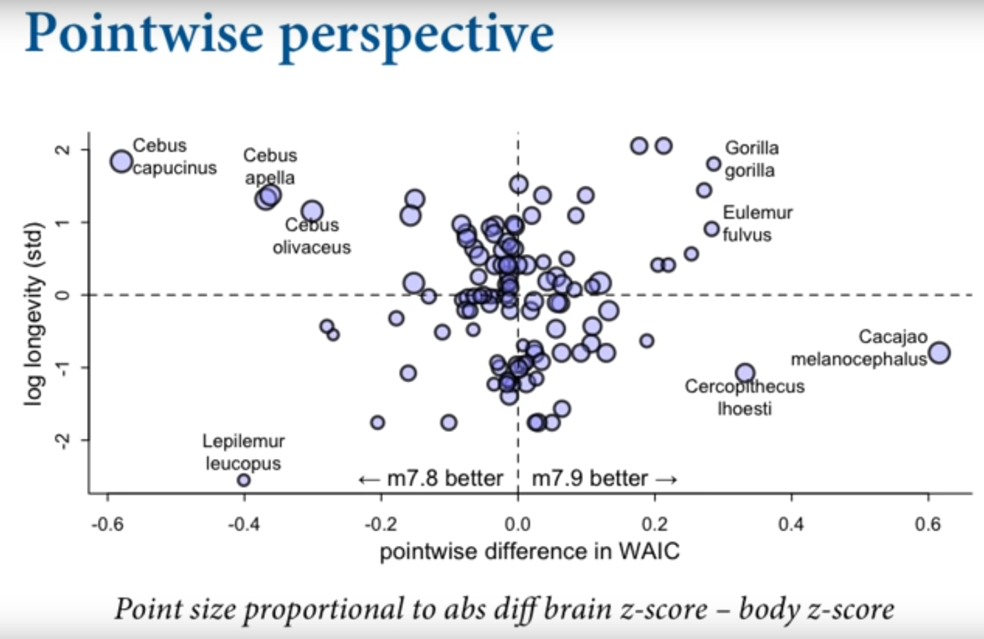
Another approach: since WAIC is point wise we can plot the difference in WAIC for each point across models
Comparing life span on Y, and point wise difference in WAIC between the two models on X
We see that the model M+B is better for some species eg. Cebus, and the simple B model is better for other species eg. Gorilla
Incredible