8 Week 8
2021-09-08 [updated: 2022-01-26]
8.1 Question 1
8.1.1 Data
DT <- data_reedfrogs()
precis(DT)
## mean sd 5.5% 94.5% histogram
## density 23.33 10.38 10.00 35 ▇▁▁▁▁▁▁▇▁▁▁▁▇
## pred NaN NA NA NA
## size NaN NA NA NA
## surv 16.31 9.88 4.58 33 ▂▇▂▁▃▁▃
## propsurv 0.72 0.27 0.29 1 ▁▁▃▁▁▂▁▅▇
writeLines(readLines(tar_read(stan_d_file_w08_model_frogs_1)))## data {
## int N;
## int survival[N];
## int density[N];
## int tank[N];
## }
## parameters {
## real sigma;
## real alpha[N];
## real alpha_bar;
## }
## transformed parameters {
## vector[N] p;
##
## for (i in 1:N) {
## p[i] = inv_logit(alpha[i]);
## }
## }
## model {
## alpha_bar ~ normal(0, 0.25);
## alpha ~ normal(alpha_bar, sigma);
## sigma ~ exponential(1);
## for (i in 1:N) {
## survival[i] ~ binomial(density[i], p[i]);
## }
## }
model_frogs_1_draws <- tar_read(stan_d_mcmc_w08_model_frogs_1)$draws()

mcmc_areas(model_frogs_1_draws, regex_pars = 'alpha')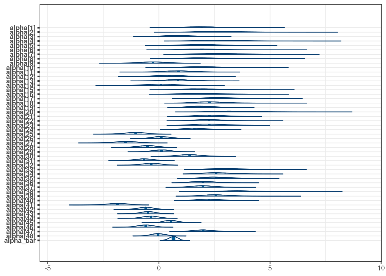
mcmc_areas(model_frogs_1_draws, regex_pars = 'p\\[')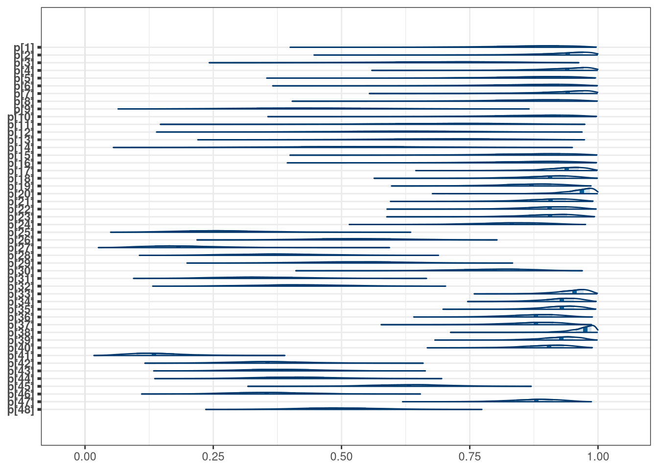
writeLines(readLines(tar_read(stan_d_file_w08_model_frogs_2)))## data {
## int N;
## int survival[N];
## int density[N];
## int tank[N];
## int predation[N];
## }
## parameters {
## real sigma;
## real alpha[N];
## real alpha_bar;
## real beta_predation;
## }
## transformed parameters {
## vector[N] p;
##
## for (i in 1:N) {
## p[i] = inv_logit(alpha[i] + beta_predation * predation[i]);
## }
## }
## model {
## alpha_bar ~ normal(0, 0.25);
## alpha ~ normal(alpha_bar, sigma);
## beta_predation ~ normal(0, 0.5);
## sigma ~ exponential(1);
## for (i in 1:N) {
## survival[i] ~ binomial(density[i], p[i]);
## }
## }
model_frogs_2_draws <- tar_read(stan_d_mcmc_w08_model_frogs_2)$draws()
mcmc_areas(model_frogs_2_draws, regex_pars = 'predation')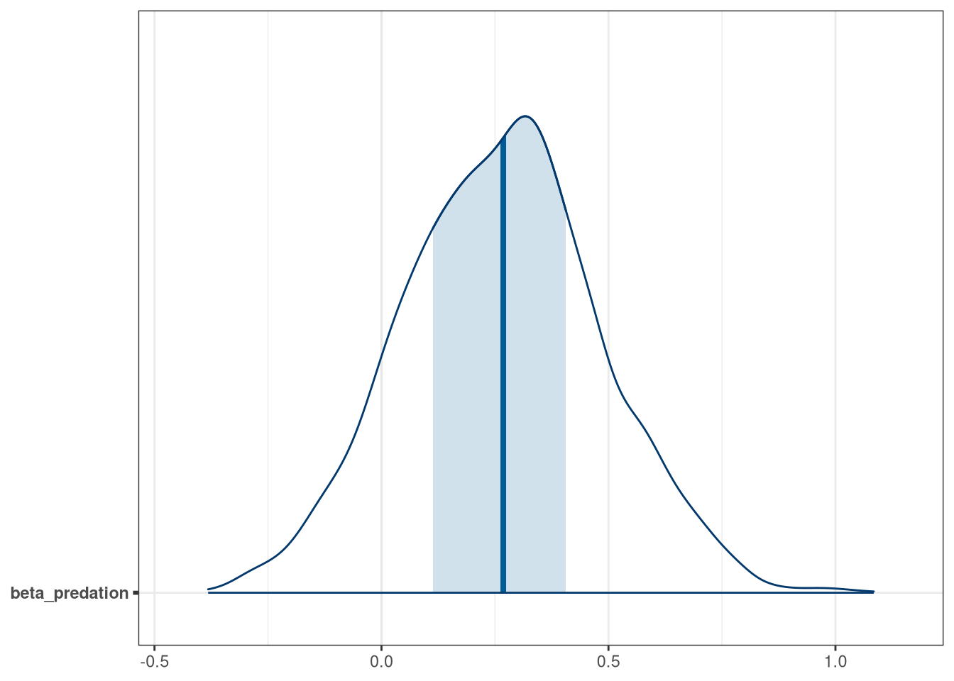
writeLines(readLines(tar_read(stan_d_file_w08_model_frogs_3)))## data {
## int N;
## int survival[N];
## int density[N];
## int tank[N];
## int size[N];
## }
## parameters {
## real sigma;
## real alpha[N];
## real alpha_bar;
## real beta_size;
## }
## transformed parameters {
## vector[N] p;
##
## for (i in 1:N) {
## p[i] = inv_logit(alpha[i] + beta_size * size[i]);
## }
## }
## model {
## alpha_bar ~ normal(0, 0.25);
## alpha ~ normal(alpha_bar, sigma);
## beta_size ~ normal(0, 0.5);
## sigma ~ exponential(1);
## for (i in 1:N) {
## survival[i] ~ binomial(density[i], p[i]);
## }
## }
model_frogs_3_draws <- tar_read(stan_d_mcmc_w08_model_frogs_3)$draws()
mcmc_areas(model_frogs_3_draws, regex_pars = 'size')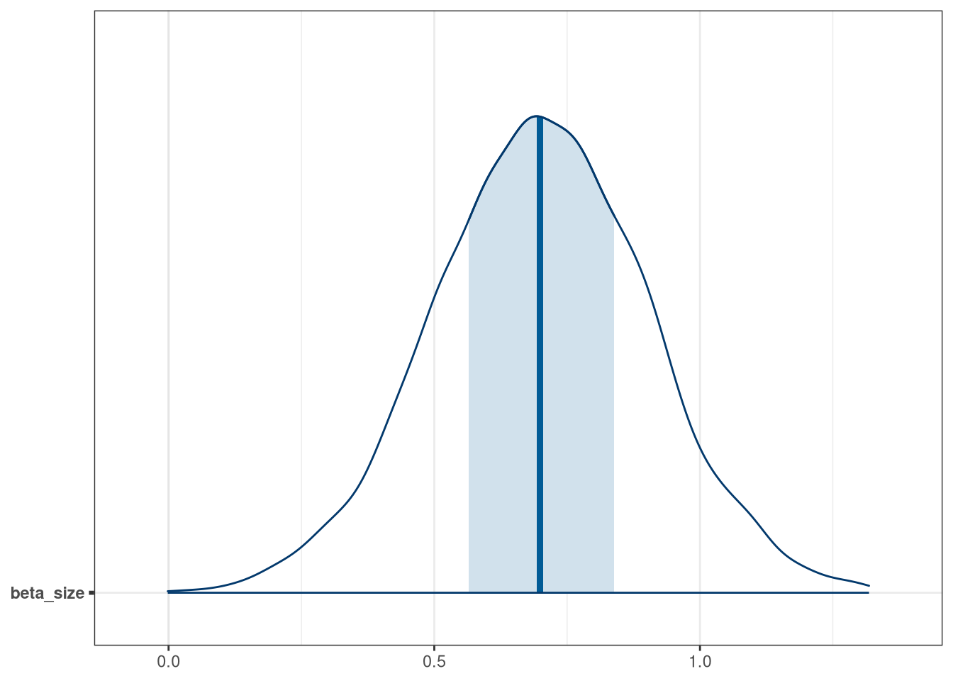
writeLines(readLines(tar_read(stan_d_file_w08_model_frogs_4)))## data {
## int N;
## int survival[N];
## int density[N];
## int tank[N];
## int size[N];
## int predation[N];
## }
## parameters {
## real sigma;
## real alpha[N];
## real alpha_bar;
## real beta_size;
## real beta_predation;
## real beta_interaction;
## }
## transformed parameters {
## vector[N] p;
##
## for (i in 1:N) {
## p[i] = inv_logit(alpha[i] + beta_size * size[i] + beta_predation * predation[i] + beta_interaction * (size[i] * predation[i]));
## }
## }
## model {
## alpha_bar ~ normal(0, 0.25);
## alpha ~ normal(alpha_bar, sigma);
## beta_size ~ normal(0, 0.5);
## beta_predation ~ normal(0, 0.5);
## beta_interaction ~ normal(0, 0.25);
## sigma ~ exponential(1);
## for (i in 1:N) {
## survival[i] ~ binomial(density[i], p[i]);
## }
## }
model_frogs_4_draws <- tar_read(stan_d_mcmc_w08_model_frogs_4)$draws()

mcmc_areas(model_frogs_4_draws, regex_pars = 'beta')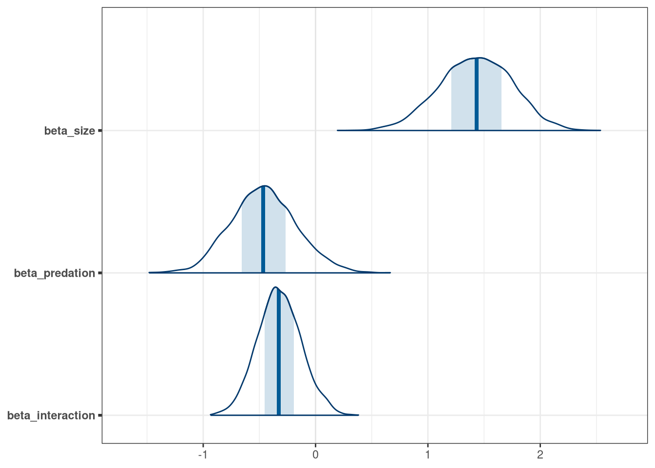
Negative influence of predation is somewhat balanced by size of tank.
8.2 Question 2
In 1980, a typical Bengali woman could have 5 or more children in her lifetime. By the year 2000, a typical Bengali woman had only 2 or 3. You’re going to look at a historical set of data, when contraception was widely available but many families chose not to use it. These data reside in
data(bangladesh)and come from the 1988 Bangladesh Fertility Survey. Each row is one of 1934 women. There are six variables, but you can focus on two of them for this practice problem: (1) district: ID number of administrative district each woman resided in (2) use.contraception: An indicator (0/1) of whether the woman was using contraception.
DT <- data_bangladesh()
precis(DT)
## mean sd 5.5% 94.5% histogram
## woman 967.500000000000000000 558.44 107.3 1827.7 ▇▇▇▇▇▇▇▇▇▅
## district 29.252843846949328821 17.80 1.0 57.0 ▇▅▇▅▅▇▅▃▅▅▅▅
## use.contraception 0.392450879007238906 0.49 0.0 1.0 ▇▁▁▁▁▁▁▁▁▅
## living.children 2.652016546018614473 1.24 1.0 4.0 ▅▃▁▃▁▇
## age.centered 0.002197880041365139 9.01 -12.6 16.4 ▅▇▇▅▃▃▂
## urban 0.290589451913133401 0.45 0.0 1.0 ▇▁▁▁▁▁▁▁▁▃
## id 967.500000000000000000 558.44 107.3 1827.7 ▇▇▇▇▇▇▇▇▇▅
## contraception 0.392450879007238906 0.49 0.0 1.0 ▇▁▁▁▁▁▁▁▁▅
## scale_age 0.000000000000000014 1.00 -1.4 1.8 ▁▇▇▅▇▃▃▂▁Now, focus on predicting use.contraception, clustered by district_id. Fit
both (1) a traditional fixed-effects model that uses an index variable for
district and (2) a multilevel model with varying intercepts for district. Plot
the predicted proportions of women in each district using contraception, for
both the fixed-effects model and the varying-effects model. That is, make a plot
in which district ID is on the horizontal axis and expected proportion using
contraception is on the vertical.Make one plot for each model, or layer them on
the same plot, as you prefer. How do the models disagree? Can you explain the
pattern of disagreement? In particular, can you explain the most extreme cases
of disagreement, both why they happen where they do and why the models reach
different inferences?
Fixed effects model
writeLines(readLines(tar_read(stan_e_file_w08_model_bang_fixed)))## data {
## // Integers for number of rows, and number of districts
## int<lower=0> N;
## int<lower=0> N_district;
##
## // District and contraception, expecting integers of length N
## int district[N];
## int contraception[N];
## }
## parameters {
## // Alpha vector matching length of number of districts
## vector[N_district] alpha;
## }
## model {
## // p vector matching length of number of districts
## vector[N] p;
##
## // Alpha is distributed normally
## alpha ~ normal(0, 1.5);
##
## // For each for in data, alpha for that row's district
## for (i in 1:N) {
## p[i] = inv_logit(alpha[district[i]]);
## }
##
## // Contraception if distributed with bernoulli, p
## contraception ~ bernoulli(p);
## }
model_bang_fixed_draws <- tar_read(stan_e_mcmc_w08_model_bang_fixed)$draws()

mcmc_areas(model_bang_fixed_draws, regex_pars = 'alpha', transformations = inv.logit)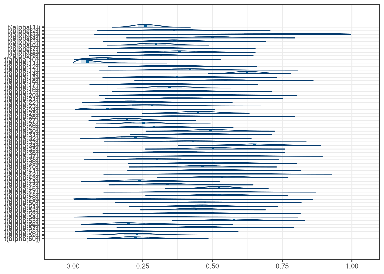
Multilevel model
writeLines(readLines(tar_read(stan_e_file_w08_model_bang_multi)))## data {
## // Integers for number of rows, and number of districts
## int<lower=0> N;
## int<lower=0> N_district;
##
## // District and contraception, expecting integers of length N
## int district[N];
## int contraception[N];
## }
## parameters {
## // Alpha vector matching length of number of districts
## vector[N_district] alpha;
## real<lower=0> sigma;
##
## // Hyper parameter alpha bar
## real alpha_bar;
## }
## model {
## // p vector matching length of number of districts
## vector[N] p;
##
## // For each for in data, alpha for that row's district
## for (i in 1:N) {
## p[i] = inv_logit(alpha[district[i]]);
## }
##
## // Hyper priors: alpha bar and sigma
## alpha_bar ~ normal(0, 1.5);
## sigma ~ exponential(1);
##
## // Priors
## // Alpha is distributed normally
## alpha ~ normal(alpha_bar, sigma);
##
## // Contraception if distributed with bernoulli, p
## contraception ~ bernoulli(p);
## }
model_bang_multi_draws <- tar_read(stan_e_mcmc_w08_model_bang_multi)$draws()

mcmc_trace(model_bang_multi_draws)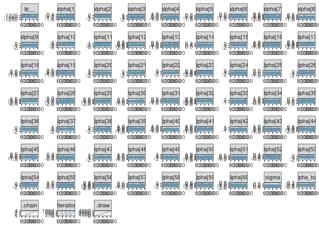
mcmc_areas(model_bang_multi_draws, regex_pars = 'alpha', transformations = inv.logit)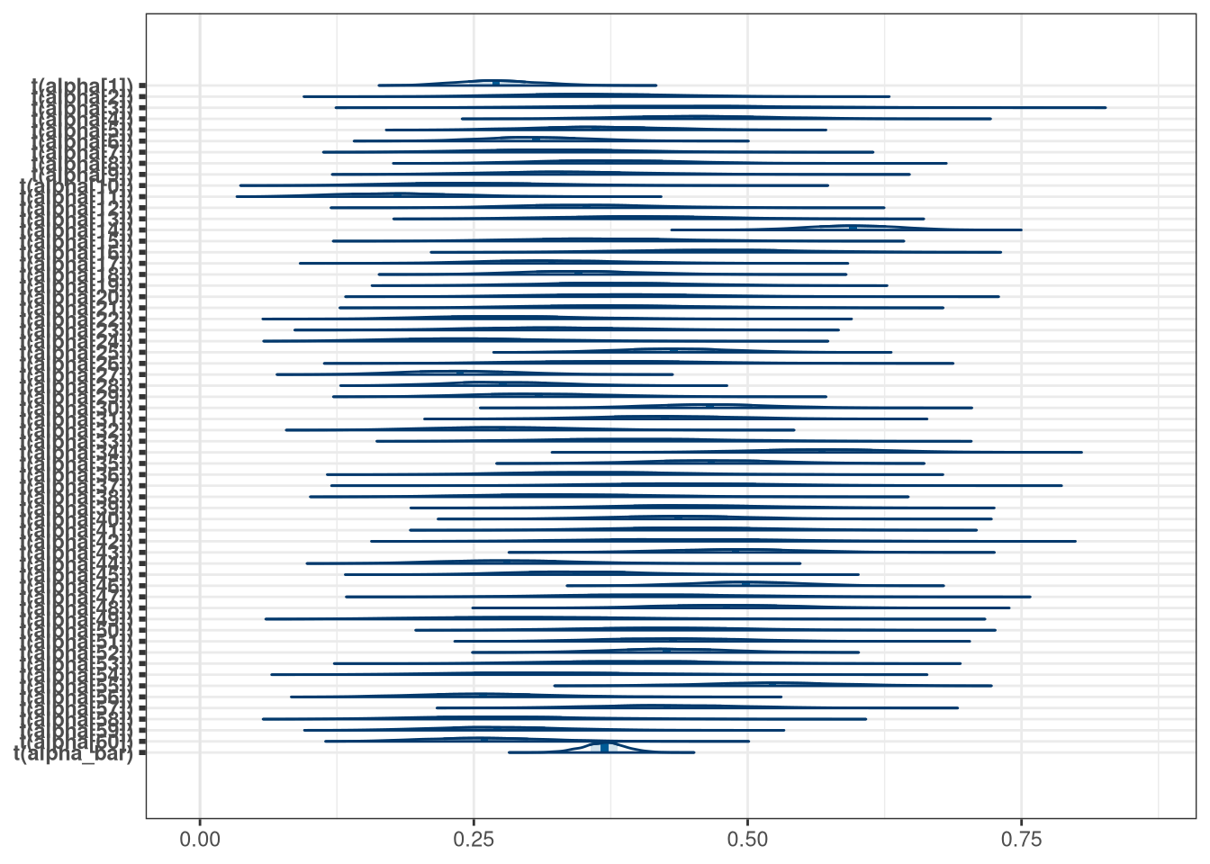
mcmc_areas(model_bang_multi_draws, pars = c('alpha_bar', 'sigma'))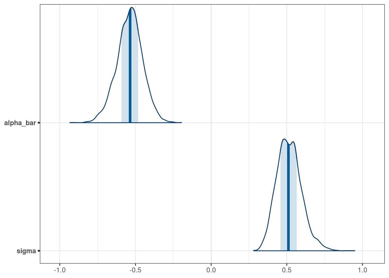
Comparison
(mcmc_areas(model_bang_fixed_draws, regex_pars = 'alpha', transformations = inv.logit) + labs(title = 'fixed')) +
    (mcmc_areas(model_bang_multi_draws, regex_pars = 'alpha\\[', transformations = inv.logit) + labs(title = 'multilevel'))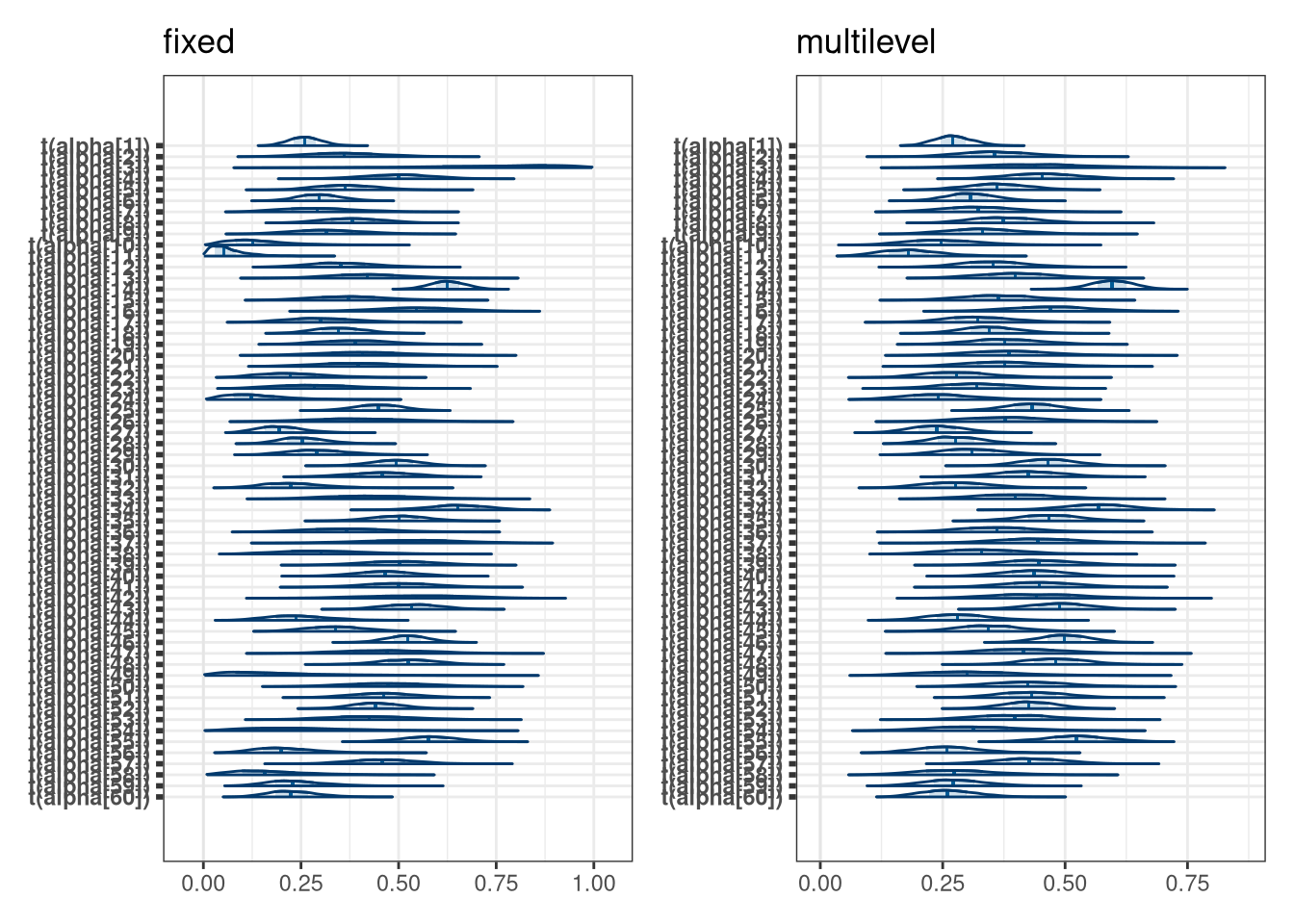
setDT(model_bang_fixed_draws)
setDT(model_bang_multi_draws)

compare <- rbindlist(list(
    melt(model_bang_fixed_draws, measure.vars = patterns('alpha'))[, model_type := 'fixed'],
    melt(model_bang_multi_draws, measure.vars = patterns('alpha'))[, model_type := 'multilevel']
), fill = TRUE)

compare[, variable := as.integer(gsub('alpha\\[|\\]', '', variable))]
## Warning in eval(jsub, SDenv, parent.frame()): NAs introduced by coercion
ggplot(compare[, .(value = mean(value)), .(variable, model_type)]) +
    geom_hline(yintercept = 0, alpha = 0.5) +
    geom_point(aes(variable, value, color = model_type)) +
    geom_line(aes(variable, value, group = model_type), alpha = 0.2) +
    scale_color_viridis_d(begin = 0.3, end = 0.8) +
    labs(x = 'district', y = 'alpha')
## Warning: Removed 1 rows containing missing values (geom_point).## Warning: Removed 1 row(s) containing missing values (geom_path).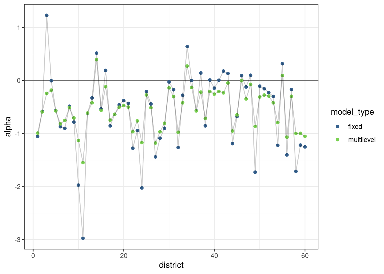
8.3 Question 3
Return to the Trolley data,
data(Trolley), from Chapter 12. Define and fit a varying intercepts model for these data. By this I mean to add an intercept parameter for the individual to the linear model. Cluster the varying intercepts on individual participants, as indicated by the unique values in the id variable. Include action, intention, and contact as before. Compare the varying intercepts model and a model that ignores individuals, using both WAIC/LOO and posterior predictions. What is the impact of individual variation in these data?
DT <- data_trolley()
precis(DT)
## mean sd 5.5% 94.5% histogram
## case NaN NA NA NA
## response 4.20 1.91 1 7 ▃▂▁▃▁▇▁▅▁▅▁▅
## order 16.50 9.29 2 31 ▇▅▇▇▅▇▂
## id NaN NA NA NA
## age 37.49 14.23 18 61 ▂▇▅▇▅▇▅▅▃▅▂▁▁
## male 0.57 0.49 0 1 ▅▁▁▁▁▁▁▁▁▇
## edu NaN NA NA NA
## action 0.43 0.50 0 1 ▇▁▁▁▁▁▁▁▁▅
## intention 0.47 0.50 0 1 ▇▁▁▁▁▁▁▁▁▇
## contact 0.20 0.40 0 1 ▇▁▁▁▁▁▁▁▁▂
## story NaN NA NA NA
## action2 0.63 0.48 0 1 ▃▁▁▁▁▁▁▁▁▇
## education 5.73 1.35 3 8 ▁▁▁▁▁▂▁▅▁▇▁▂▁▂
## individual 166.00 95.56 19 313 ▇▇▇▇▇▇▅
writeLines(readLines(tar_read(stan_c_file_w08_model_trolley)))## data {
## int N;
## int K;
## int response[N];
## int action[N];
## int intention[N];
## int contact[N];
##
## }
## parameters {
## // Cut points are the positions of responses along cumulative odds
## ordered[K] cutpoints;
## real beta_action;
## real beta_intention;
## real beta_contact;
## real beta_intention_contact;
## real beta_intention_action;
## }
## transformed parameters {
## vector[N] phi;
##
## for (i in 1:N) {
## phi[i] = beta_action * action[i] + beta_contact * contact[i] + beta_intention * intention[i] + beta_intention_contact * intention[i] * contact[i] + beta_intention_action * intention[i] * action[i];
## }
## }
## model {
## response ~ ordered_logistic(phi, cutpoints);
## cutpoints ~ normal(0, 1.5);
## beta_action ~ normal(0, 0.5);
## beta_contact ~ normal(0, 0.5);
## beta_intention ~ normal(0, 0.5);
## }
## generated quantities {
## vector[N] log_lik;
## for (i in 1:N) {
## log_lik[i] = ordered_logistic_lpmf(response[i] | phi[i], cutpoints);
## }
## }
model_trolley <- tar_read(stan_c_mcmc_w08_model_trolley)
model_trolley_draws <- model_trolley$draws()

mcmc_areas(model_trolley_draws, regex_pars = 'cutpoints')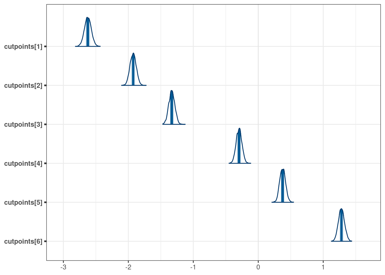
mcmc_areas(model_trolley_draws, regex_pars = 'beta')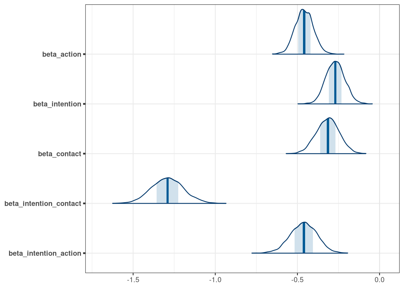
options(cmdstanr_draws_format = "draws_array")
model_trolley_loo <- model_trolley$loo()
options(cmdstanr_draws_format = "draws_df")
writeLines(readLines(tar_read(stan_c_file_w08_model_trolley_multi)))## data {
## int N;
## int K;
## int response[N];
## int action[N];
## int intention[N];
## int contact[N];
## int individual[N];
## int N_individual;
## }
## parameters {
## // Cut points are the positions of responses along cumulative odds
## ordered[K] cutpoints;
## real beta_action;
## real beta_intention;
## real beta_contact;
## real beta_intention_contact;
## real beta_intention_action;
## real alpha_bar;
## real sigma;
## vector[N_individual] alpha;
## }
## transformed parameters {
## vector[N] phi;
##
## for (i in 1:N) {
## phi[i] = alpha[individual[i]] + beta_action * action[i] +
## beta_contact * contact[i] + beta_intention * intention[i] +
## beta_intention_contact * intention[i] * contact[i] +
## beta_intention_action * intention[i] * action[i];
## }
## }
## model {
## // Hyper parameter priors
## alpha_bar ~ normal(0, 1.5);
## sigma ~ exponential(1);
##
## // Priors
## alpha ~ normal(alpha_bar, sigma);
##
## response ~ ordered_logistic(phi, cutpoints);
## cutpoints ~ normal(0, 1.5);
## beta_action ~ normal(0, 0.5);
## beta_contact ~ normal(0, 0.5);
## beta_intention ~ normal(0, 0.5);
## }
## generated quantities {
## vector[N] log_lik;
## for (i in 1:N) {
## log_lik[i] = ordered_logistic_lpmf(response[i] | phi[i], cutpoints);
## }
## }
model_trolley_multi <- tar_read(stan_c_mcmc_w08_model_trolley_multi)
model_trolley_multi_draws <- model_trolley_multi$draws()

mcmc_areas(model_trolley_multi_draws, regex_pars = 'cutpoints')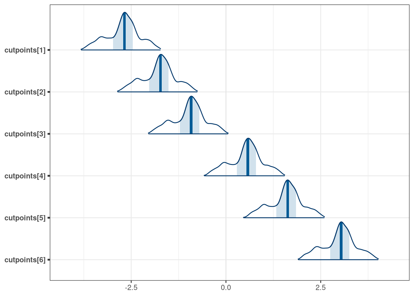
mcmc_areas(model_trolley_multi_draws, regex_pars = 'beta')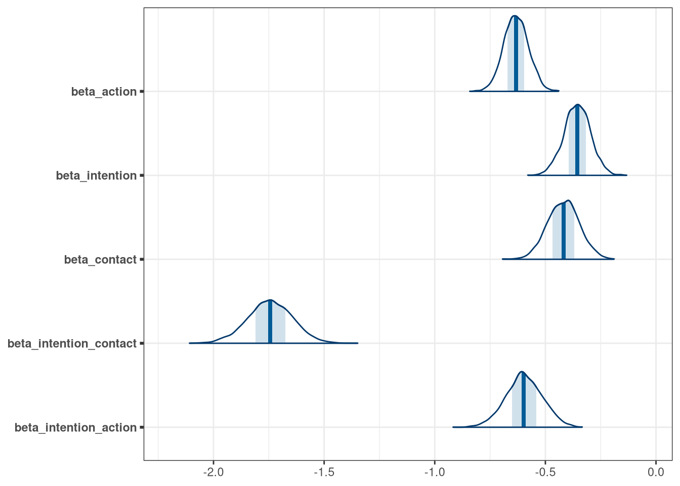
options(cmdstanr_draws_format = "draws_array")
model_trolley_multi_loo <- model_trolley_multi$loo()
options(cmdstanr_draws_format = "draws_df")
col_patterns <- '^beta|^alpha|^sigma|^cutpoints'
setDT(model_trolley_draws)
setDT(model_trolley_multi_draws)

precis(model_trolley_draws[, .SD, .SDcols = patterns(col_patterns)])
## 6 vector or matrix parameters hidden. Use depth=2 to show them.## mean sd 5.5% 94.5% histogram
## beta_action -0.46 0.055 -0.54 -0.37 ▁▁▁▃▇▇▂▁▁▁
## beta_intention -0.27 0.058 -0.36 -0.18 ▁▁▁▅▇▅▂▁▁▁
## beta_contact -0.32 0.069 -0.43 -0.21 ▁▁▁▂▅▇▇▃▁▁▁
## beta_intention_contact -1.29 0.097 -1.44 -1.13 ▁▁▁▁▃▅▇▇▇▃▂▁▁▁▁
## beta_intention_action -0.46 0.081 -0.59 -0.34 ▁▁▁▁▃▅▇▇▅▂▁▁▁
precis(model_trolley_multi_draws[, .SD, .SDcols = patterns(col_patterns)])## 337 vector or matrix parameters hidden. Use depth=2 to show them.## mean sd 5.5% 94.5% histogram
## beta_action -0.63 0.056 -0.72 -0.54 ▁▁▂▇▇▅▁▁▁
## beta_intention -0.36 0.060 -0.45 -0.26 ▁▁▁▃▇▇▃▁▁▁
## beta_contact -0.42 0.072 -0.54 -0.30 ▁▁▁▂▇▇▇▃▁▁▁
## beta_intention_contact -1.74 0.101 -1.91 -1.58 ▁▁▁▃▇▅▁▁▁
## beta_intention_action -0.60 0.082 -0.73 -0.46 ▁▁▁▁▂▅▇▇▅▂▁▁▁
## alpha_bar 1.01 0.437 0.26 1.72 ▁▁▁▂▂▂▇▇▅▂▂▁▁
## sigma 1.92 0.082 1.80 2.06 ▁▁▁▁▃▇▇▅▃▁▁▁▁▁
compared <- loo_compare(model_trolley_loo, model_trolley_multi_loo)
print(compared, simplify = FALSE)
## elpd_diff se_diff elpd_loo se_elpd_loo p_loo se_p_loo looic
## model2 0.0 0.0 -15529.0 89.8 356.8 4.7 31058.0
## model1 -2935.7 86.8 -18464.7 40.5 11.1 0.1 36929.5
## se_looic
## model2 179.6
## model1 81.1