10 Lecture 01 - 2019

A framework for developing + using statistical golems

Bayesian data analysis
- uses probability to describe uncertainty
- “count all the ways data can happen, according to assumptions and the assumptions with more ways consistent with the data are more plausible”
Multilevel models
- Models within models
- Avoids averaging
- …
Model comparison
- Compare meaningful (not null) models
- Caution: over fitting

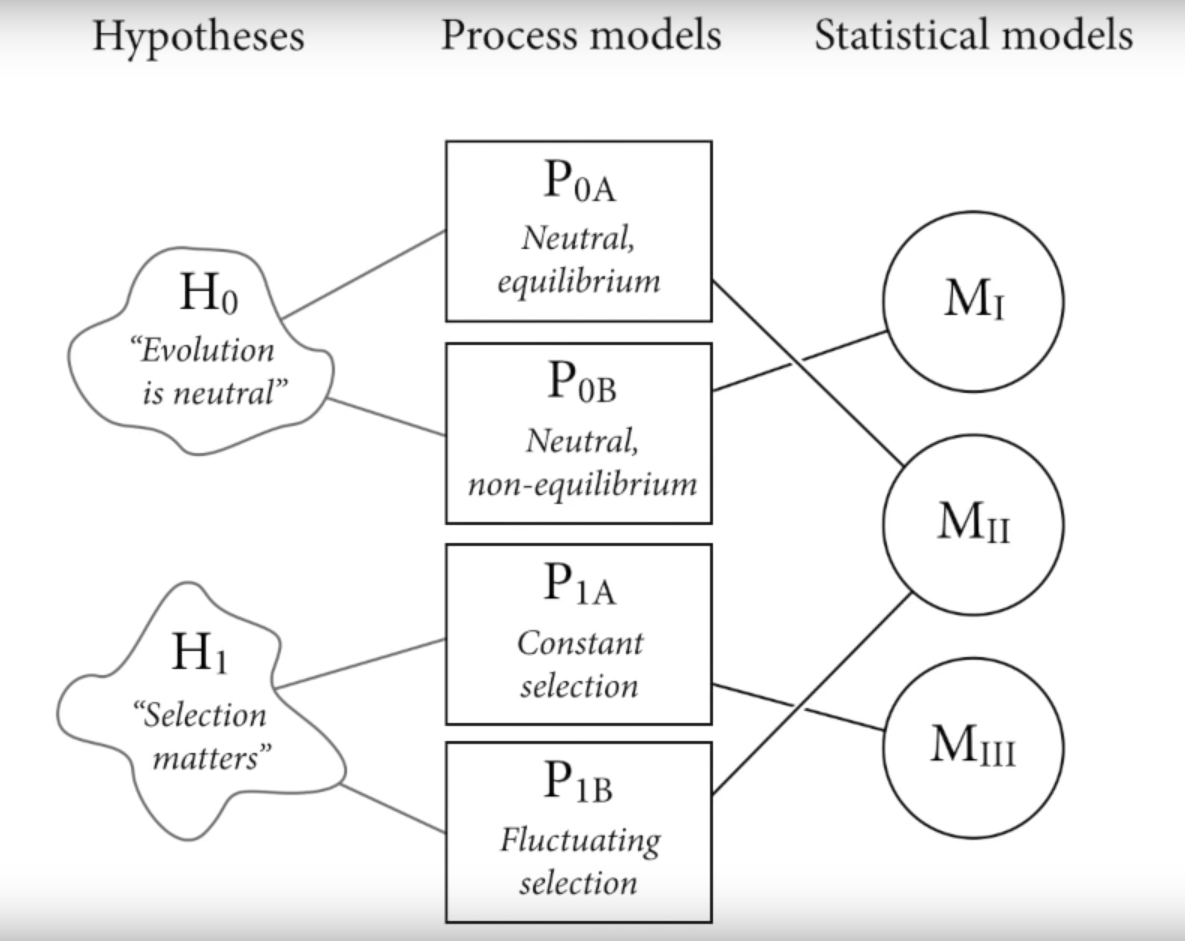
10.1 Hypotheses - Process Models - Statistical Models

Any statistical model M can correspond to multiple process models

Any hypothesis H may correspond to multiple process models

Any statistical model may correspond to multiple hypothesis

Small world: models have assumptions, Bayesian models fit optimally

Large world: real world, no guarantee of optimality

Setup

4 marbles, either black or white, with replacement

Possibilities (5) therefore: WWWW, BWWW, BBWW, BBBW, BBBB

Observation: BWB

Calculate

Given 3 observations, there are 4 choices, for a total of 64 possibilities

Given we observed both a white and a black marble, possibilities WWWW and BBBB are not valid

At each branch, there are 3 possibilities it can be white and 1 possibility it can be black

Bayesian is additive, at each branch just sum the possibility

BWWW: 3 = 1 * 3 * 1

BBWW: 8 = 2 * 2 * 2

BBBW: 9 = 3 * 1 * 3

Using new information

New information is directly integrated into the old information, therefore just multiply it through

So if we take another measure of B, multiply the property through

BWWW: 3 * 1 = 3

BBWW: 8 * 2 = 16

BBBW: 9 * 3 = 27

Using other information

Factory says B measures are rare, but minimum of 1 per bag

           Factory info

WWWW 0 since we observed a B

BWWW: 3

BBWW: 2

BBBW: 1

BBBB 0 since we observed a W

Multiply it through

BWWW: 3 * 3 = 9

BBWW: 16 * 2 = 32

BBBW: 1 * 27 = 27

Counts get huge - therefore we normalize them giving us probabilities (0-1)

Probability theory is just normalized counting