20 Lecture 11 - 2019

Flat distributions have the highest entropy and have many more ways that they can be realized

20.1 Maximum entropy

Distribution with the largest entropy is the distribution most consistent with stated assumptions

For parameters: helps understand priors. What are the constraints that make a prior reasonable?

For observations: way to understand likelihood

Solving for the posterior = getting the distribution that is as flat as possible and consistent with data within constraints

Highest entropy answer = distance to the truth is smaller

20.1.1 Distributions

Constraints	Maxent distribution	Example
Real value in interval	Uniform	Bird proportions
Real value, finite variance	Gaussian	Coin flip
Binary events, fixed probability	Binomial	Marble drawing, globe tossing
Non negative real, has mean	Exponential	Amount of time until event

20.2 Generalized linear model

Connect linear model to outcome variable

1. Pick outcome distribution
2. Model its parameter using links to linear models
3. Compute posterior

Extends to multivariate relationships and non-linear responses

Building blocks of multilevel models

Very common and widely applicable

20.2.1 Picking a distribution

Mostly exponential family because all are maximum entropy interpretations and arise from natural processes

Do not pick by looking at a histogram - no way an aggregate histogram of outcomes unconditional on something else is going to have a relevant distribution

Just use principles.

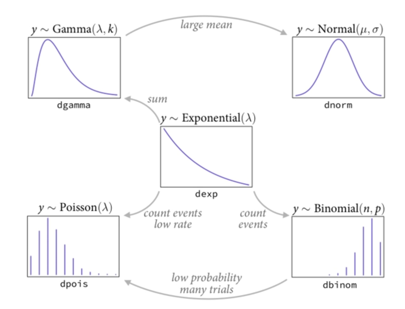
• Exponential: non negative real. Lambda is a rate and the mean is 1/lambda
• Binomial: count events emerging from an exponential distribution
• Poisson: count events, low rate
• Gamma: sum of exponential
• Normal: gamma with large mean

Tide prediction machine - complex “parameters” at the bottom. “Can understand models if you resist the urge to understand parameters”

20.2.2 Types of outcomes

Distances and durations

• Exponential
• Gamma

Counts

• Poisson
• Binomial
• Multinomial
• Geometry

Monsters

• Ranks, ordered categories

Mixtures

• Beta binomial
• Gamma-poisson
• Etc

20.2.3 Model parameters with a link function

Yi ~ Normal(mu, sigma)

mu ~ alpha + beta * X

Linear regressions and only linear regressions have the same scientific units for both the outcome variable and parameters for the mean

Another example - binomial

Count: Y ~ Binomial(N, p) (unit is count of something)

Probability: P ? alpha + beta * X (unit less)

We need some function

f(p) = alpha + beta * X

20.3 Binomial distribution

Counts of a specific event out of n possible trials

min: 0, max: n

Constant expected value

Maxent: binomial

y ~ Binomial(n, p)

count successes is distribution binomially with n trials and p probability of success

20.3.1 Link

Goal is to map linear model to [0, 1]

y ~ Binomial(n, p)

logit(p) = alpha + beta * x

logit is the log odds

Given this link function, priors on the logit scale are the not same shape as priors on the probability scale

Prosocial monkey example

y ~ Binomial(n, p)

logit(p) = alpha[actor] + beta[treatment] * Treatment

precis(m)

a[1] … a[7] a are the different chimps, the posterior means are on the logit scale

b[1] … b[4] b are the treatments, the average log odd deviations after chimp handedness has been considered

Investigating

1. extract samples
2. inv_logit to transform to probability score
3. precis

It’s really hard to understand just using the precis output therefore

1. Plot on the outcome scale with link = posterior predictive sampling

Controlling for handedness here isn’t because of the backdoor criterion. Handedness = noise, controlling for it gives us a more precise criteria