5 Week 5
2021-09-03 [updated: 2022-01-26]
5.1 Question 1
Consider the
data(Wines2012)data table. These data are expert ratings of 20 different French and American wines by 9 different French and American judges.
5.1.1 Data
Your goal is to model score, the subjective rating assigned by each judge to each wine. I recommend standardizing it. In this first problem, consider only variation among judges and wines. Construct index variables of judge and wine and then use these index variables to construct a linear regression model.
DT <- data_wines()

n_index_judge <- DT[, uniqueN(index_judge)]
n_index_wine <- DT[, uniqueN(index_wine)]
n_rows <- DT[, .N]
5.1.2 Prior predictive simulation
writeLines(readLines(tar_read(stan_file_w05_q1_prior)))## data {
## int<lower=0> N;
## int<lower=0> N_judges;
## int<lower=0> N_wines;
## }
## parameters{
## real alpha;
## vector[N_judges] beta_judge;
## vector[N_wines] beta_wine;
## real<lower=0> sigma;
## }
## model{
## sigma ~ exponential(1);
## beta_wine ~ normal(0, 0.5);
## beta_judge ~ normal(0, 0.5);
## alpha ~ normal(0, 0.2);
## }
q1_prior_draws <- tar_read(stan_mcmc_w05_q1_prior)$draws()

mcmc_areas(q1_prior_draws, regex_pars = 'judge')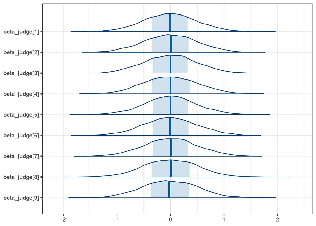
mcmc_areas(q1_prior_draws, regex_pars = 'wine')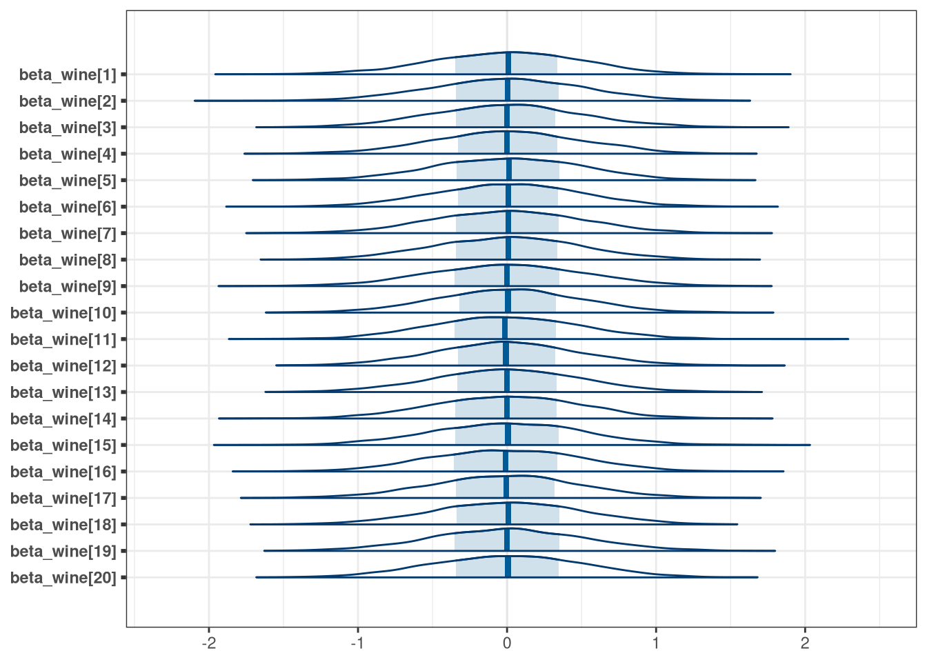
Justify your priors. You should end up with 9 judge parameters and 20 wine parameters.
Given the parameters are scaled, the prior predictive plots show scaled wine scores mostly between -2 and 2. Since we do not have any prior knowledge about how this relationship (positive/negative slopes), we are satisfied with this relatively conservative prior.
5.1.3 Model
Use ulam instead of quap to build this model, and be sure to check the chains for convergence. If you’d rather build the model directly in Stan or PyMC3, go ahead. I just want you to use Hamiltonian Monte Carlo instead of quadratic approximation.
writeLines(readLines(tar_read(stan_file_w05_q1)))## data {
## int<lower=0> N;
## int<lower=0> N_judges;
## int<lower=0> N_wines;
## int index_judge[N];
## int index_wine[N];
## vector[N] scale_score;
## }
## parameters{
## real alpha;
## vector[N_judges] beta_judge;
## vector[N_wines] beta_wine;
## real<lower=0> sigma;
## }
## model{
## alpha ~ normal(0, 0.2);
## beta_wine ~ normal(0, 0.5);
## beta_judge ~ normal(0, 0.5);
## sigma ~ exponential(1);
##
## vector[N] mu;
## mu = beta_wine[index_wine] + beta_judge[index_judge];
## scale_score ~ normal(mu, sigma);
## }
q1_draws <- tar_read(stan_mcmc_w05_q1)$draws()
setDT(q1_draws)
How do you interpret the variation among individual judges and individual wines? Do you notice any patterns, just by plotting the differences? Which judges gave the highest/lowest ratings? Which wines were rated worst/ best on average?
# Judges
precis(q1_draws, depth = 2)[3:11,]
## mean sd 5.5% 94.5% histogram
## beta_judge[1] -0.54 0.19 -0.861 -0.233 ▁▁▁▁▂▃▇▇▇▅▂▁▁▁▁
## beta_judge[2] -0.34 0.19 -0.644 -0.038 ▁▁▁▁▂▃▇▇▇▅▂▁▁▁
## beta_judge[3] 0.80 0.20 0.490 1.109 ▁▁▃▇▇▂▁▁
## beta_judge[4] 0.13 0.20 -0.179 0.452 ▁▁▁▃▇▅▂▁
## beta_judge[5] -0.65 0.19 -0.963 -0.343 ▁▁▁▁▂▃▇▇▇▃▂▁▁▁
## beta_judge[6] 0.48 0.20 0.162 0.792 ▁▁▁▅▇▃▁▁
## beta_judge[7] -0.28 0.20 -0.592 0.035 ▁▁▁▁▃▅▇▇▇▃▂▁▁▁
## beta_judge[8] 0.21 0.20 -0.106 0.527 ▁▁▂▇▇▂▁▁▁
## beta_judge[9] 0.21 0.19 -0.089 0.519 ▁▁▂▇▇▃▁▁▁
melt(q1_draws, measure.vars = patterns('beta_judge'))[, .(mean_score = mean(value)), variable][order(-mean_score)]## variable mean_score
## 1: beta_judge[3] 0.80
## 2: beta_judge[6] 0.48
## 3: beta_judge[9] 0.21
## 4: beta_judge[8] 0.21
## 5: beta_judge[4] 0.13
## 6: beta_judge[7] -0.28
## 7: beta_judge[2] -0.34
## 8: beta_judge[1] -0.54
## 9: beta_judge[5] -0.65
mcmc_areas(q1_draws, regex_pars = 'judge')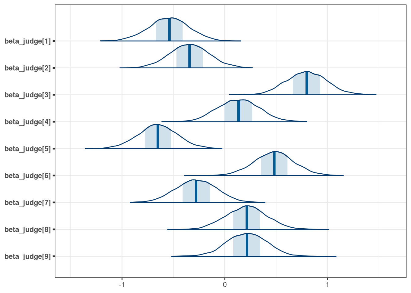
# Wines
precis(q1_draws, depth = 2)[12:31,]
## mean sd 5.5% 94.5% histogram
## beta_wine[1] 0.1175 0.25 -0.282 0.526 ▁▁▂▅▇▇▂▁▁▁
## beta_wine[2] 0.2271 0.26 -0.187 0.630 ▁▁▁▃▇▇▅▂▁▁
## beta_wine[3] -0.1017 0.26 -0.514 0.314 ▁▁▂▅▇▅▂▁▁▁
## beta_wine[4] 0.2406 0.26 -0.174 0.648 ▁▁▁▃▇▇▅▂▁▁
## beta_wine[5] 0.0668 0.26 -0.351 0.477 ▁▁▁▂▇▇▅▂▁▁▁
## beta_wine[6] -0.0117 0.26 -0.431 0.407 ▁▁▁▃▇▇▃▁▁▁
## beta_wine[7] -0.0901 0.26 -0.515 0.302 ▁▁▂▅▇▇▂▁▁▁
## beta_wine[8] -0.1886 0.26 -0.608 0.232 ▁▁▁▃▇▇▃▁▁▁
## beta_wine[9] -0.1196 0.24 -0.516 0.271 ▁▁▂▅▇▅▂▁▁
## beta_wine[10] -0.1401 0.26 -0.554 0.273 ▁▁▁▁▂▇▇▅▂▁▁
## beta_wine[11] 0.0858 0.26 -0.329 0.509 ▁▁▁▂▅▇▅▂▁▁▁
## beta_wine[12] 0.4641 0.26 0.035 0.869 ▁▁▁▂▅▇▅▂▁▁▁
## beta_wine[13] -0.3145 0.26 -0.716 0.091 ▁▁▁▂▅▇▅▂▁▁▁
## beta_wine[14] 0.2234 0.27 -0.200 0.642 ▁▁▁▃▇▇▅▂▁▁
## beta_wine[15] 0.0963 0.26 -0.311 0.515 ▁▁▁▂▅▇▅▂▁▁▁
## beta_wine[16] -0.0234 0.26 -0.424 0.389 ▁▁▁▁▅▇▇▃▁▁▁
## beta_wine[17] 0.0051 0.26 -0.420 0.432 ▁▁▁▃▇▇▃▁▁▁
## beta_wine[18] -0.1674 0.26 -0.591 0.261 ▁▁▁▃▇▇▅▂▁▁
## beta_wine[19] -0.7246 0.26 -1.137 -0.303 ▁▁▁▂▇▇▅▂▁▁
## beta_wine[20] 0.3215 0.25 -0.068 0.717 ▁▁▁▂▅▇▇▂▁▁
melt(q1_draws, measure.vars = patterns('beta_wine'))[, .(mean_score = mean(value)), variable][order(-mean_score)]## variable mean_score
## 1: beta_wine[12] 0.4641
## 2: beta_wine[20] 0.3215
## 3: beta_wine[4] 0.2406
## 4: beta_wine[2] 0.2271
## 5: beta_wine[14] 0.2234
## 6: beta_wine[1] 0.1175
## 7: beta_wine[15] 0.0963
## 8: beta_wine[11] 0.0858
## 9: beta_wine[5] 0.0668
## 10: beta_wine[17] 0.0051
## 11: beta_wine[6] -0.0117
## 12: beta_wine[16] -0.0234
## 13: beta_wine[7] -0.0901
## 14: beta_wine[3] -0.1017
## 15: beta_wine[9] -0.1196
## 16: beta_wine[10] -0.1401
## 17: beta_wine[18] -0.1674
## 18: beta_wine[8] -0.1886
## 19: beta_wine[13] -0.3145
## 20: beta_wine[19] -0.7246
mcmc_areas(q1_draws, regex_pars = 'wine')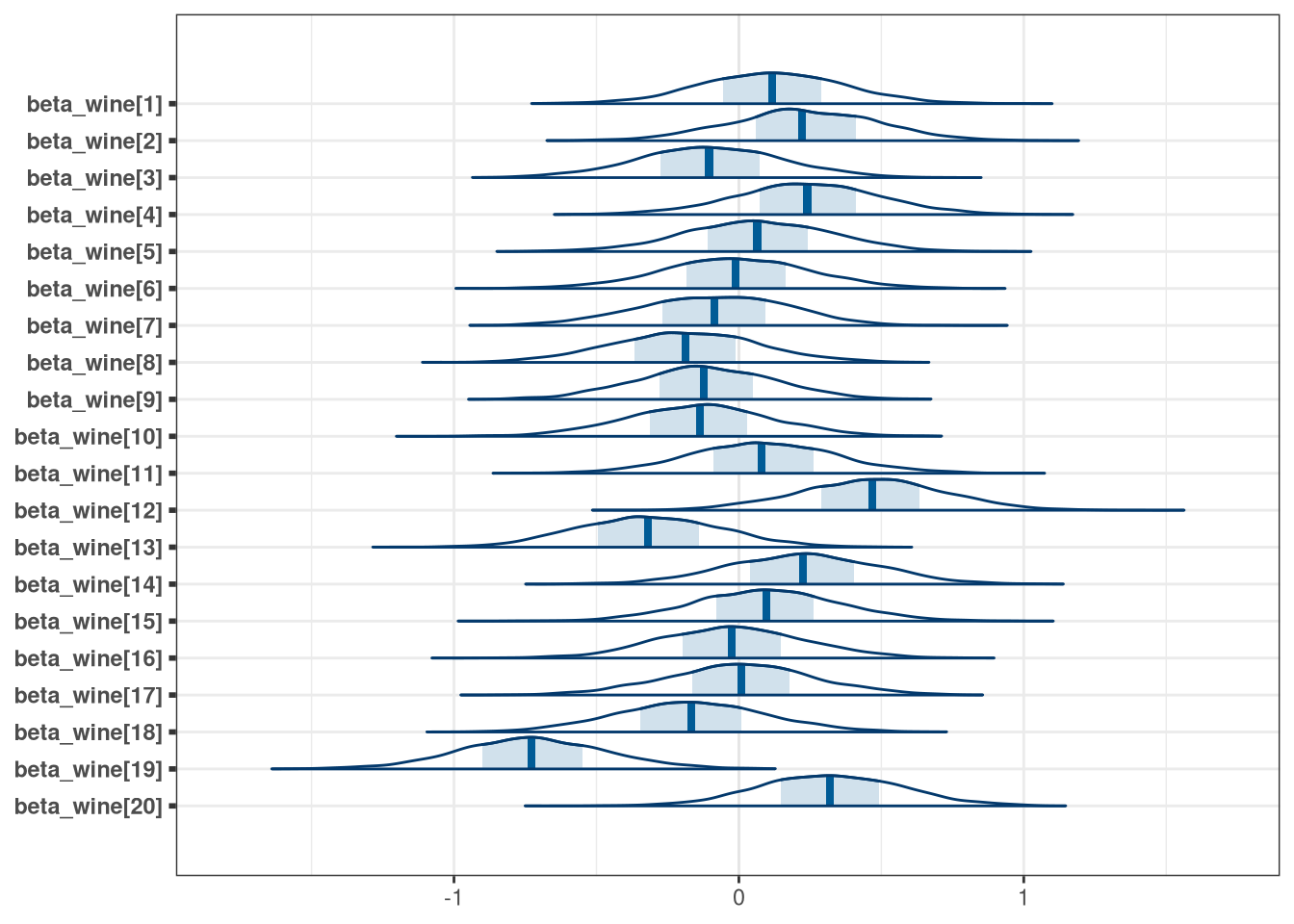
Accounting for judges, most wines are scored with similar distributions. Wine 19 however was particularly poorly scored. Judges, however, have much more variable scoring with three individuals (judges 1, 2, 5) entirely or almost entirely scoring lower than other judges. The worst scoring judge was judge 5.
5.2 Question 2
Now consider three features of the wines and judges: (1) flight: Whether the wine is red or white. (2) wine.amer: Indicator variable for American wines. (3) judge.amer: Indicator variable for American judges. Use indicator or index variables to model the influence of these features on the scores. Omit the individual judge and wine index variables from Problem 1. Do not include interaction effects yet. Again use ulam, justify your priors, and be sure to check the chains.
5.2.1 Data
DT <- data_wines()

n_index_flight <- DT[, uniqueN(flight)]
n_index_wine_american <- DT[, uniqueN(index_wine_american)]
n_index_judge_american <- DT[, uniqueN(index_judge_american)]
n_rows <- DT[, .N]

q2_data <- c(
    as.list(DT[, .(scale_score = as.numeric(scale_score),
                                 index_flight,
                                 index_wine_american,
                                 index_judge_american)]),
    N_flights = n_index_flight,
    N_wine_american = n_index_wine_american,
    N_judge_american = n_index_judge_american,
    N = n_rows
)
5.2.2 Priors
writeLines(readLines(tar_read(stan_file_w05_q2_prior)))## data {
## int<lower=0> N;
## int<lower=0> N_flights;
## int<lower=0> N_wine_american;
## int<lower=0> N_judge_american;
## }
## parameters{
## real alpha;
## vector[N_flights] beta_flights;
## vector[N_wine_american] beta_wine_american;
## vector[N_judge_american] beta_judge_american;
## real<lower=0> sigma;
## }
## model{
## alpha ~ normal(0, 0.2);
## beta_flights ~ normal(0, 0.5);
## beta_wine_american ~ normal(0, 0.5);
## beta_judge_american ~ normal(0, 0.5);
## sigma ~ exponential(1);
## }
q2_prior_draws <- tar_read(stan_mcmc_w05_q2_prior)$draws()

mcmc_areas(q2_prior_draws, regex_pars = 'flights')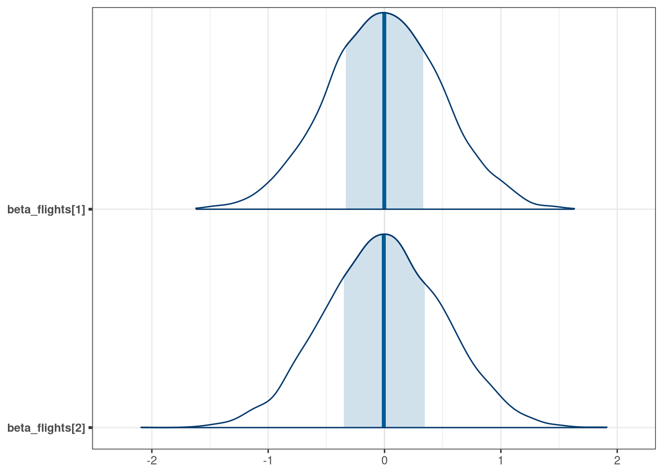
mcmc_areas(q2_prior_draws, regex_pars = 'judge')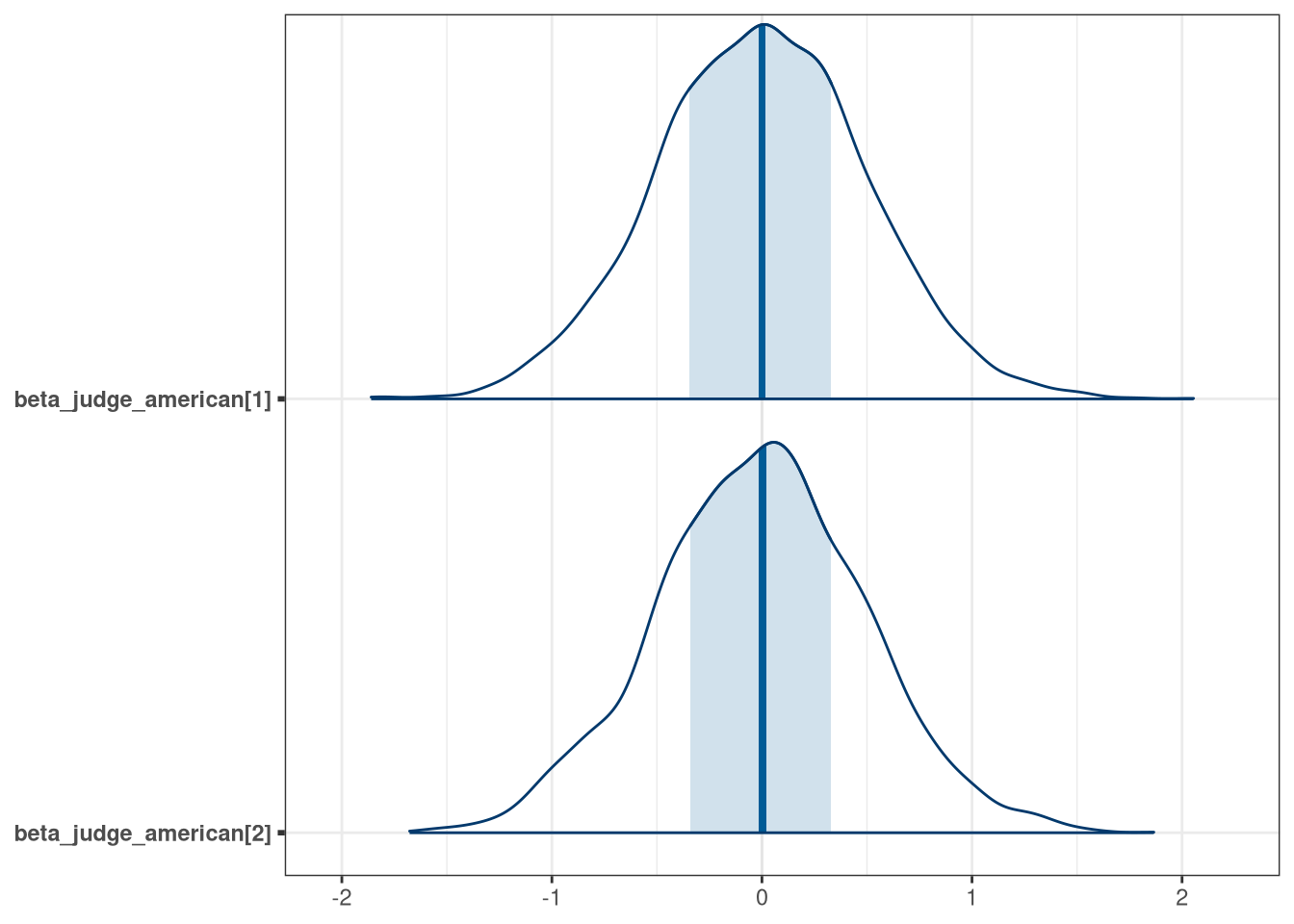
mcmc_areas(q2_prior_draws, regex_pars = 'wine')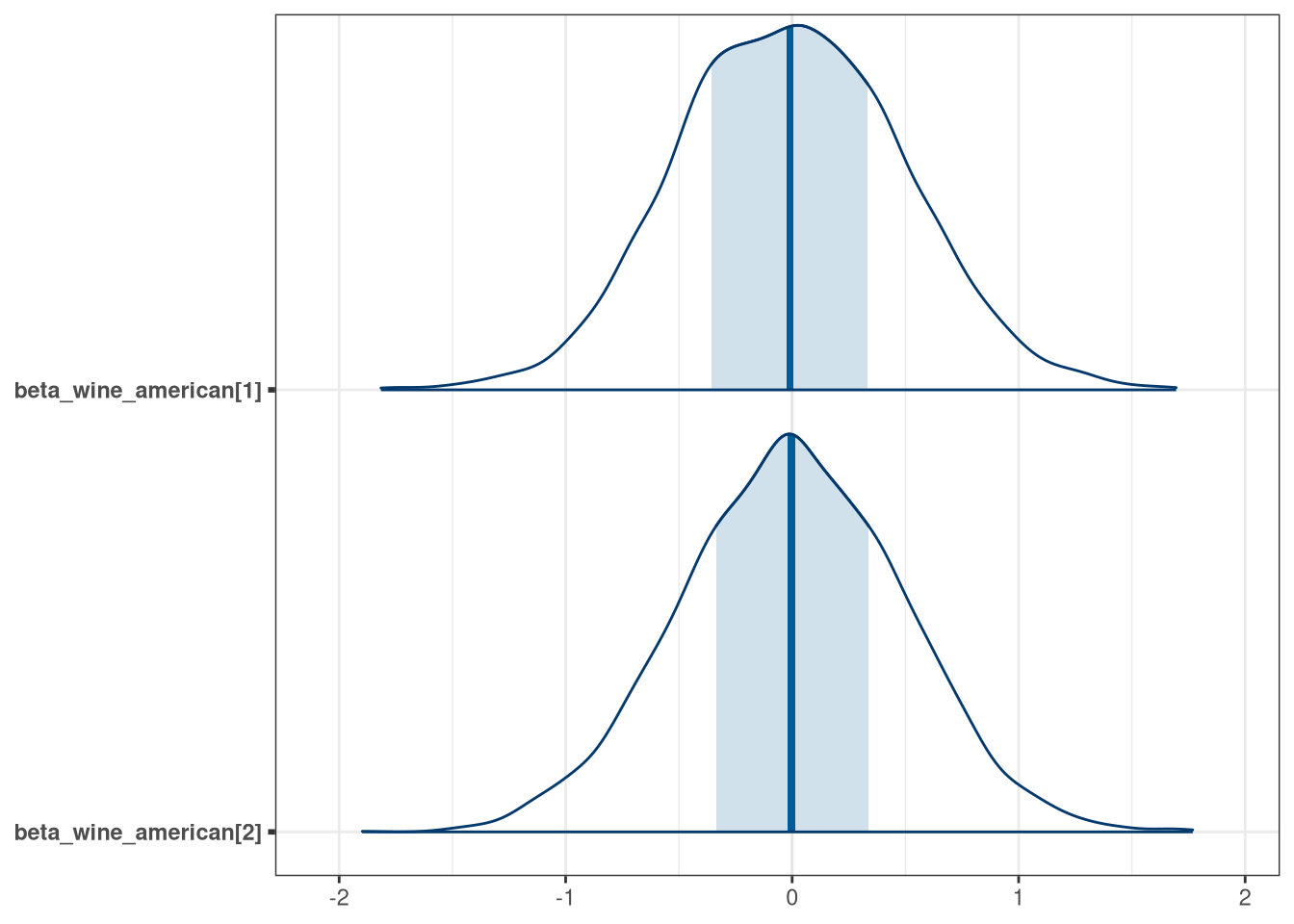
5.2.3 Model
writeLines(readLines(tar_read(stan_file_w05_q2)))## data {
## int<lower=0> N;
## int<lower=0> N_flights;
## int<lower=0> N_wine_american;
## int<lower=0> N_judge_american;
##
## int index_flight[N];
## int index_wine_american[N];
## int index_judge_american[N];
##
## vector[N] scale_score;
## }
## parameters{
## real alpha;
## vector[N_flights] beta_flights;
## vector[N_wine_american] beta_wine_american;
## vector[N_judge_american] beta_judge_american;
## real<lower=0> sigma;
## }
## model{
## alpha ~ normal(0, 0.2);
## beta_flights ~ normal(0, 0.5);
## beta_wine_american ~ normal(0, 0.5);
## beta_judge_american ~ normal(0, 0.5);
## sigma ~ exponential(1);
##
## vector[N] mu;
## mu = beta_flights[index_flight] + beta_wine_american[index_wine_american] + beta_judge_american[index_judge_american];
## scale_score ~ normal(mu, sigma);
## }
q2 <- tar_read(stan_mcmc_w05_q2)
q2_draws <- q2$draws()

q2$summary()
## # A tibble: 9 × 10
## variable mean median sd mad q5 q95 rhat ess_bulk
## <chr> <dbl> <dbl> <dbl> <dbl> <dbl> <dbl> <dbl> <dbl>
## 1 lp__ -9.24e+1 -9.20e+1 2.04 1.92 -96.2 -89.7 1.00 1746.
## 2 alpha 8.61e-4 -1.84e-4 0.198 0.196 -0.312 0.336 1.00 3101.
## 3 beta_flights[… -2.04e-3 -9.90e-4 0.297 0.295 -0.501 0.484 1.00 1876.
## 4 beta_flights[… -5.52e-3 -1.04e-2 0.298 0.303 -0.483 0.489 1.00 1929.
## 5 beta_wine_ame… -8.69e-2 -8.85e-2 0.303 0.302 -0.575 0.403 1.00 1730.
## 6 beta_wine_ame… 9.67e-2 1.02e-1 0.301 0.302 -0.406 0.589 1.00 1847.
## 7 beta_judge_am… -1.16e-1 -1.14e-1 0.296 0.295 -0.590 0.361 1.00 1864.
## 8 beta_judge_am… 1.21e-1 1.20e-1 0.291 0.290 -0.347 0.602 1.00 1762.
## 9 sigma 1.00e+0 9.99e-1 0.0534 0.0529 0.918 1.09 1.00 3052.
## # … with 1 more variable: ess_tail <dbl>
mcmc_trace(q2_draws)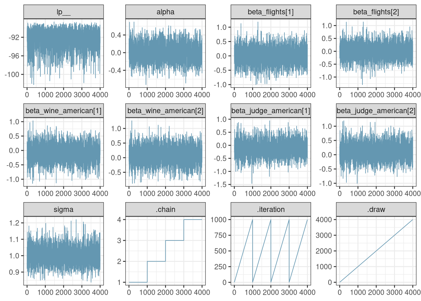
# Recall:
DT[, .N, .(flight, index_flight)]
## flight index_flight N
## 1: white 1 90
## 2: red 2 90
DT[, .N, .(judge.amer, index_judge_american)]## judge.amer index_judge_american N
## 1: 0 1 80
## 2: 1 2 100
DT[, .N, .(wine.amer, index_wine_american)]## wine.amer index_wine_american N
## 1: 1 1 108
## 2: 0 2 72
labs <- c(
    'beta_flights[1]' = 'White Wine',
    'beta_flights[2]' = 'Red Wine',
    'beta_wine_american[1]' = 'French Wine',
    'beta_wine_american[2]' = 'American Wine',
    'beta_judge_american[1]' = 'American Judge',
    'beta_judge_american[2]' = 'French Judge'
)
mcmc_areas(q2_draws, regex_pars = 'flight') + scale_y_discrete(labels = labs)
## Scale for 'y' is already present. Adding another scale for 'y', which will
## replace the existing scale.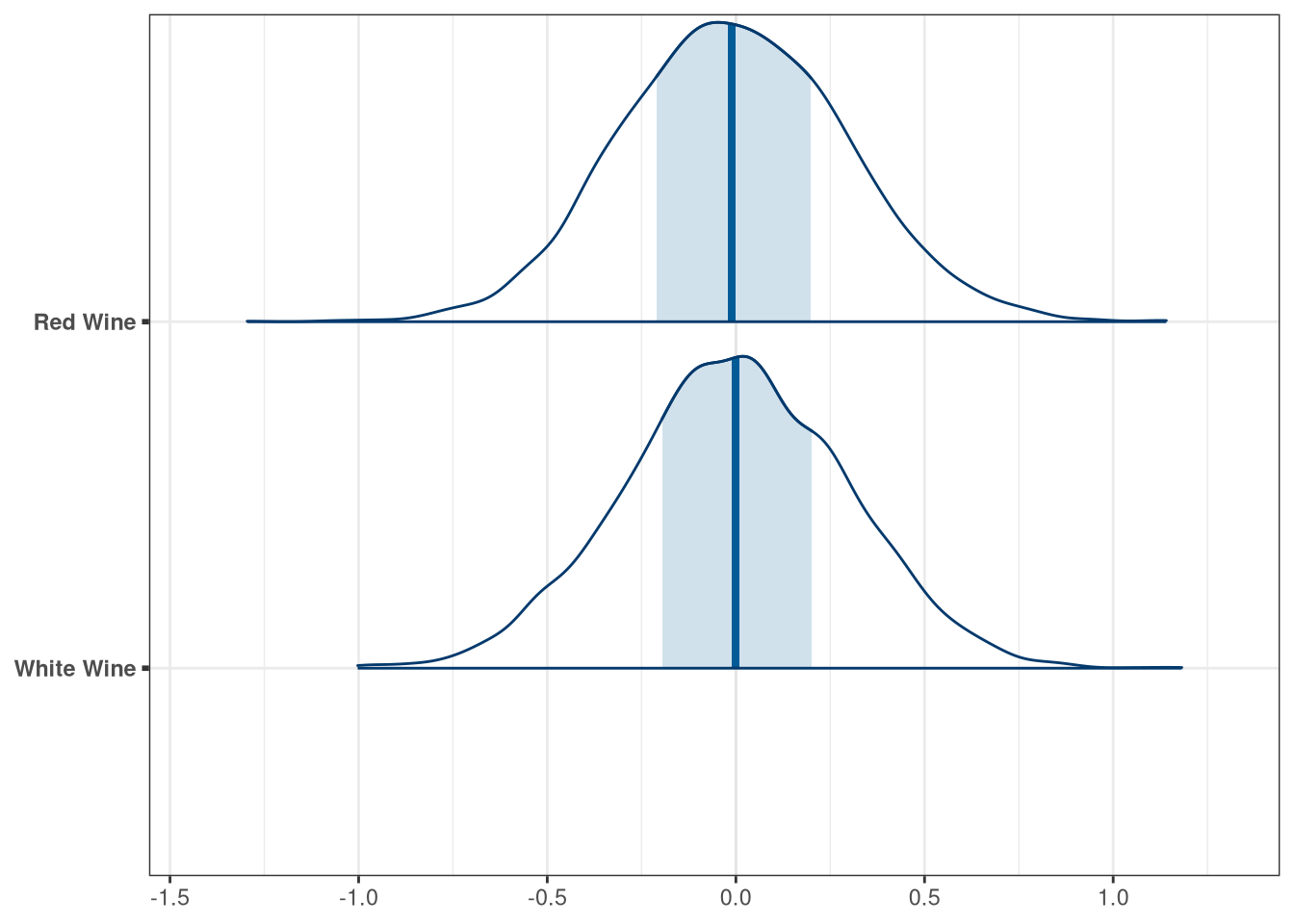
mcmc_areas(q2_draws, regex_pars = 'judge') + scale_y_discrete(labels = labs)## Scale for 'y' is already present. Adding another scale for 'y', which will
## replace the existing scale.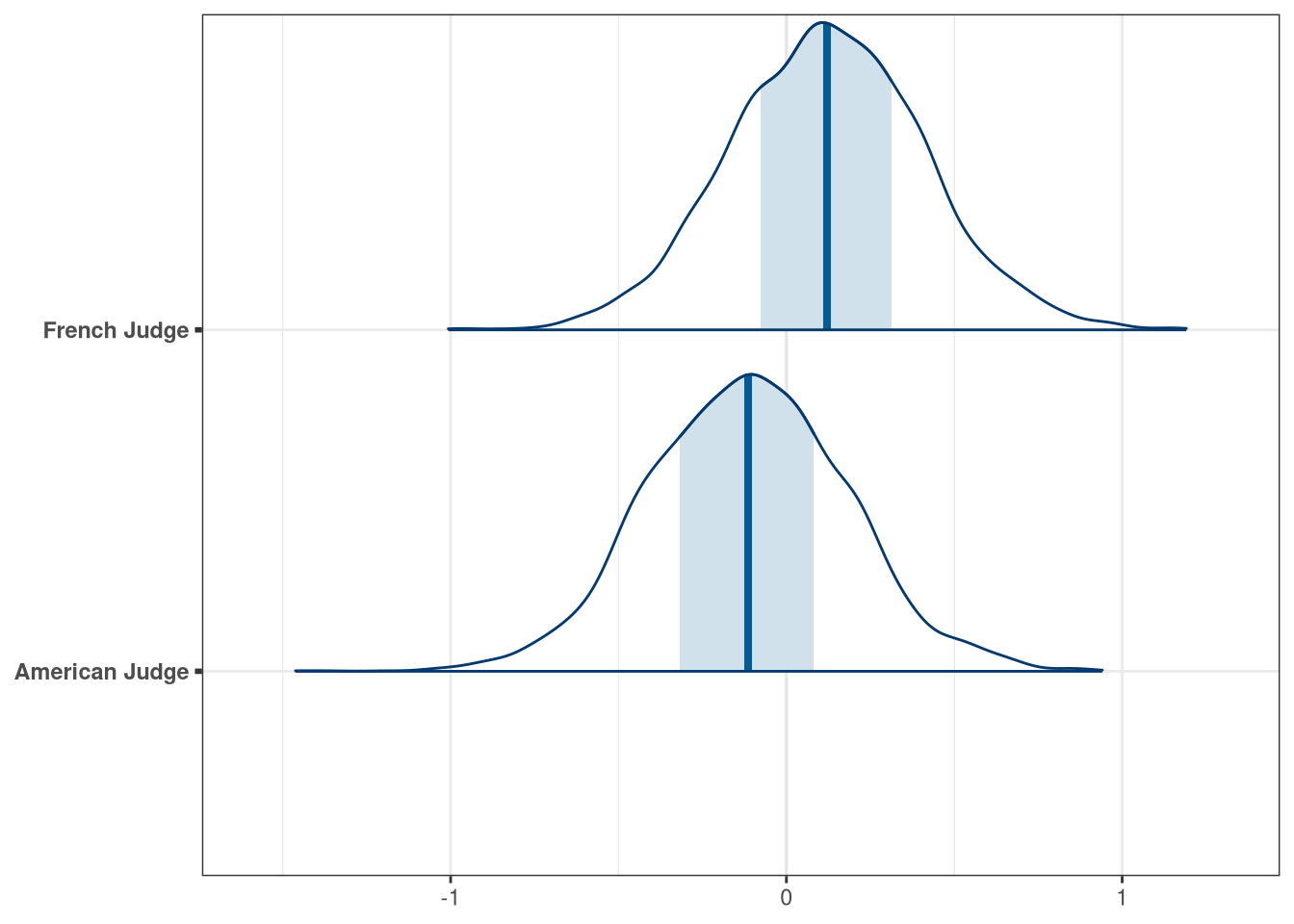
mcmc_areas(q2_draws, regex_pars = 'wine') + scale_y_discrete(labels = labs)## Scale for 'y' is already present. Adding another scale for 'y', which will
## replace the existing scale.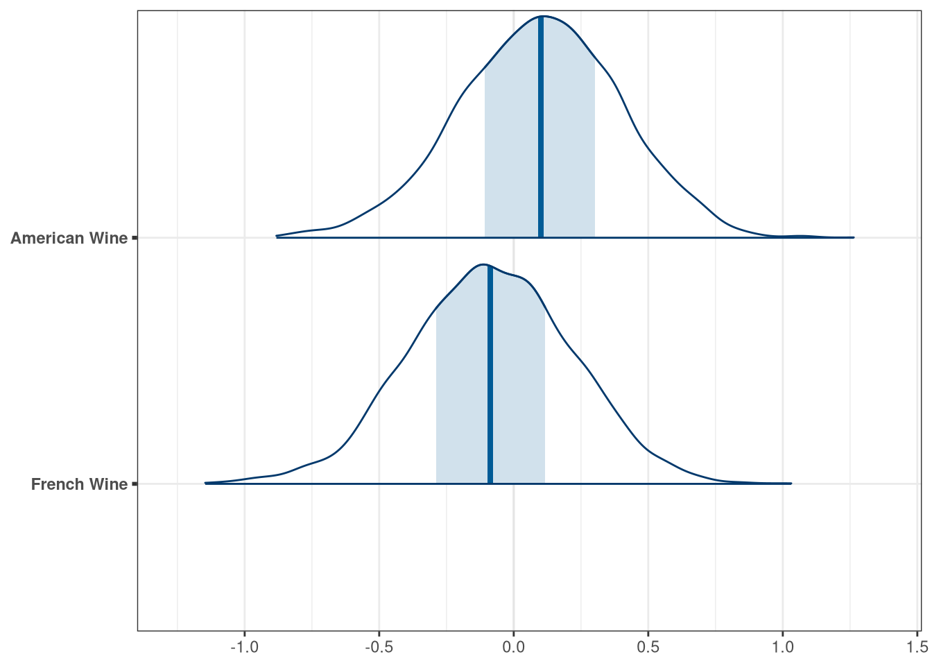
5.3 Question 3
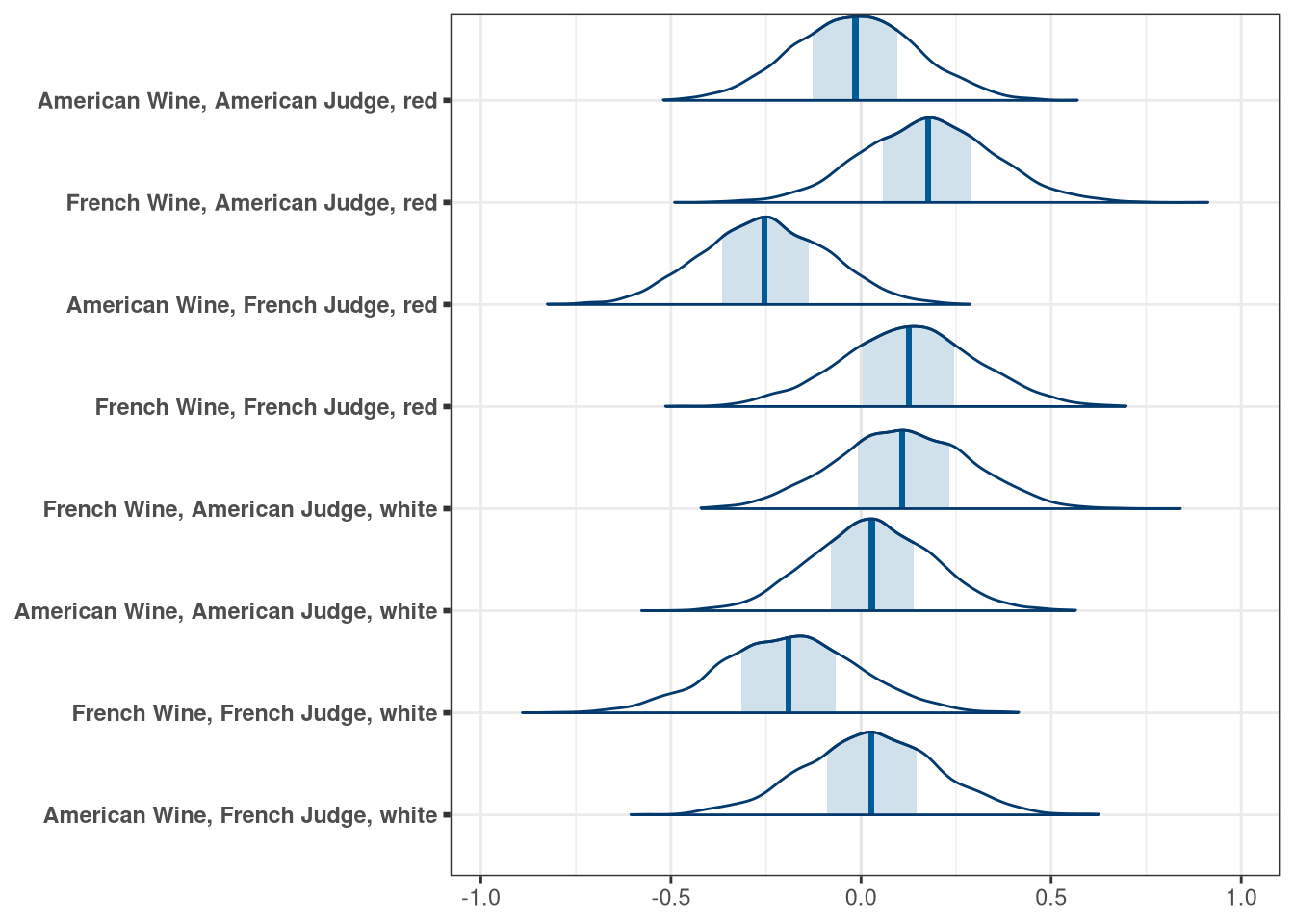
Now consider two-way interactions among the three features. You should end up with three different interaction terms in your model. These will be easier to build, if you use indicator variables. Again use ulam, justify your priors, and be sure to check the chains. Explain what each interaction means. Be sure to interpret the model’s predictions on the outcome scale (mu, the expected score), not on the scale of individual parameters. You can use link to help with this, or just use your knowledge of the linear model instead. What do you conclude about the features and the scores? Can you relate the results of your model(s) to the individual judge and wine inferences from Problem 1?
5.3.1 Data
DT <- data_wines()
n_index_interactions <- DT[, uniqueN(index_interactions)]

q3_data <- c(
    as.list(DT[, .(scale_score = as.numeric(scale_score),
                                 index_interactions)]),
    N_interactions = n_index_interactions,
    N = n_rows
)
5.3.2 Model
writeLines(readLines(tar_read(stan_file_w05_q3)))## data {
## int<lower=0> N;
## int<lower=0> N_interactions;
##
## int index_interactions[N];
##
## vector[N] scale_score;
## }
## parameters{
## real alpha;
## vector[N_interactions] beta_interactions;
## real<lower=0> sigma;
## }
## model{
## alpha ~ normal(0, 0.2);
## beta_interactions ~ normal(0, 0.25);
## sigma ~ exponential(1);
##
## vector[N] mu;
## mu = alpha + beta_interactions[index_interactions];
##
## scale_score ~ normal(mu, sigma);
## }
q3 <- tar_read(stan_mcmc_w05_q3)
q3_draws <- q3$draws()

q3$summary()
## # A tibble: 11 × 10
## variable mean median sd mad q5 q95 rhat ess_bulk
## <chr> <dbl> <dbl> <dbl> <dbl> <dbl> <dbl> <dbl> <dbl>
## 1 lp__ -9.25e+1 -9.22e+1 2.23 2.07 -96.7 -89.5 1.00 1640.
## 2 alpha 1.86e-3 1.15e-3 0.101 0.0991 -0.164 0.168 1.00 3164.
## 3 beta_interac… 2.58e-2 2.68e-2 0.176 0.174 -0.266 0.317 1.00 5526.
## 4 beta_interac… -1.91e-1 -1.90e-1 0.185 0.183 -0.503 0.113 1.00 6850.
## 5 beta_interac… 2.91e-2 2.83e-2 0.158 0.161 -0.228 0.289 1.00 4941.
## 6 beta_interac… 1.10e-1 1.08e-1 0.177 0.179 -0.183 0.402 1.00 5471.
## 7 beta_interac… 1.26e-1 1.27e-1 0.179 0.178 -0.174 0.421 1.00 6705.
## 8 beta_interac… -2.52e-1 -2.54e-1 0.166 0.167 -0.524 0.0208 1.00 6633.
## 9 beta_interac… 1.76e-1 1.77e-1 0.174 0.173 -0.105 0.461 1.00 6188.
## 10 beta_interac… -1.45e-2 -1.48e-2 0.164 0.165 -0.283 0.261 1.00 4721.
## 11 sigma 9.91e-1 9.90e-1 0.0520 0.0535 0.909 1.08 1.00 8835.
## # … with 1 more variable: ess_tail <dbl>
mcmc_trace(q3_draws)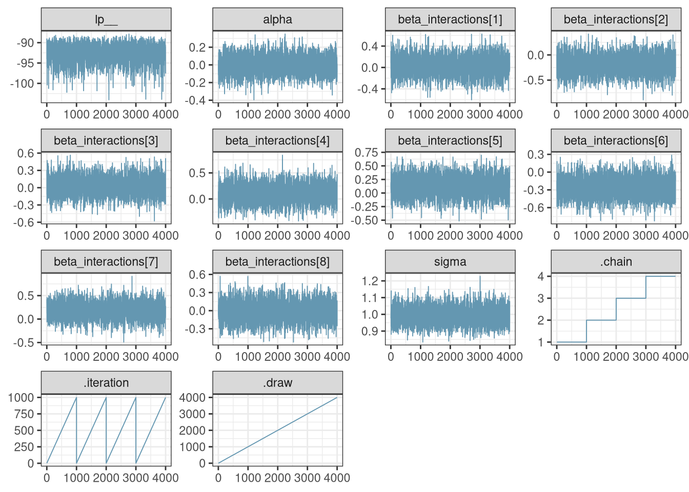
DT[, judge_char := ifelse(judge.amer == 0, 'French Judge', 'American Judge')]
DT[, wine_char := ifelse(wine.amer == 0, 'French Wine', 'American Wine')]

labs <- DT[, .(.GRP, paste(.BY, collapse = ', ')), by = .(wine_char, judge_char, as.character(flight))][, .(GRP, V2)]
labs <- setNames(labs$V2, paste0('beta_interactions[', labs$GRP, ']'))
mcmc_areas(q3_draws, regex_pars = 'interaction') + scale_y_discrete(labels = labs)
## Scale for 'y' is already present. Adding another scale for 'y', which will
## replace the existing scale.