3 Week 3

2021-08-25 [updated: 2022-01-26]

3.1 Overview

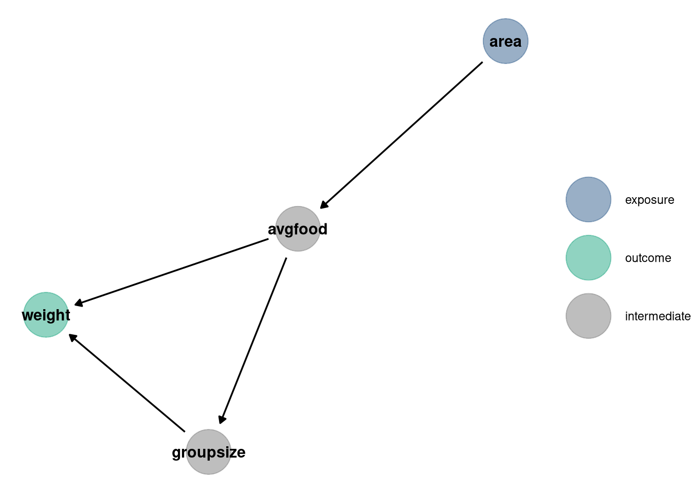
All three problems below are based on the same data. The data in data(foxes) are 116 foxes from 30 different urban groups in England. These foxes are like street gangs. Group size varies from 2 to 8 individuals. Each group maintains its own (almost exclusive) urban territory. Some territories are larger than others. The area variable encodes this information. Some territories also have more avgfood than others. We want to model the weight of each fox. For the problems below, assume this DAG

3.1.1 Setup

# DAG
dag <- dagify(
    weight ~ groupsize + avgfood,
    groupsize ~ avgfood,
    avgfood ~ area,
    exposure = 'area',
    outcome = 'weight'
)

dag_plot(dag)

3.2 Question 1

Use a model to infer the total causal influence of area on weight. Would increasing the area available to each fox make it heavier (healthier)? You might want to standardize the variables. Regardless, use prior predictive simulation to show that your model’s prior predictions stay within the possible outcome range.

3.2.1 Workings

Area on weight

scale(weight) ~ dnorm(mu, sigma)
mu <- a + b * (scale(area))
a: intercept
when weight and area are scaled, the expected intercept is 0
therefore
a ~ dnorm(0, 0.5)

b: beta, rate of change given one unit of increase in area
b ~ dnorm(0, 1)

sigma: standard deviation
uniform prior
sigma ~ dunif(0, 50)

3.2.2 Model

data(foxes)

foxes$scale_area <- scale(foxes$area)
foxes$scale_weight <- scale(foxes$weight)

m1 <- quap(
    alist(
        scale_weight ~ dnorm(mu, sigma),
        mu <- a + bArea * scale_area,
        a ~ dnorm(0, 0.05),
        bArea ~ dnorm(0, 0.5),
        sigma ~ dunif(0, 50)
    ), 
    data = foxes
)

3.2.3 Prior predictive simulation

prior <- extract.prior(m1)
l <- link(m1, post = prior, data = list(scale_area = c(-2, 2)))
plot_link(l, 20)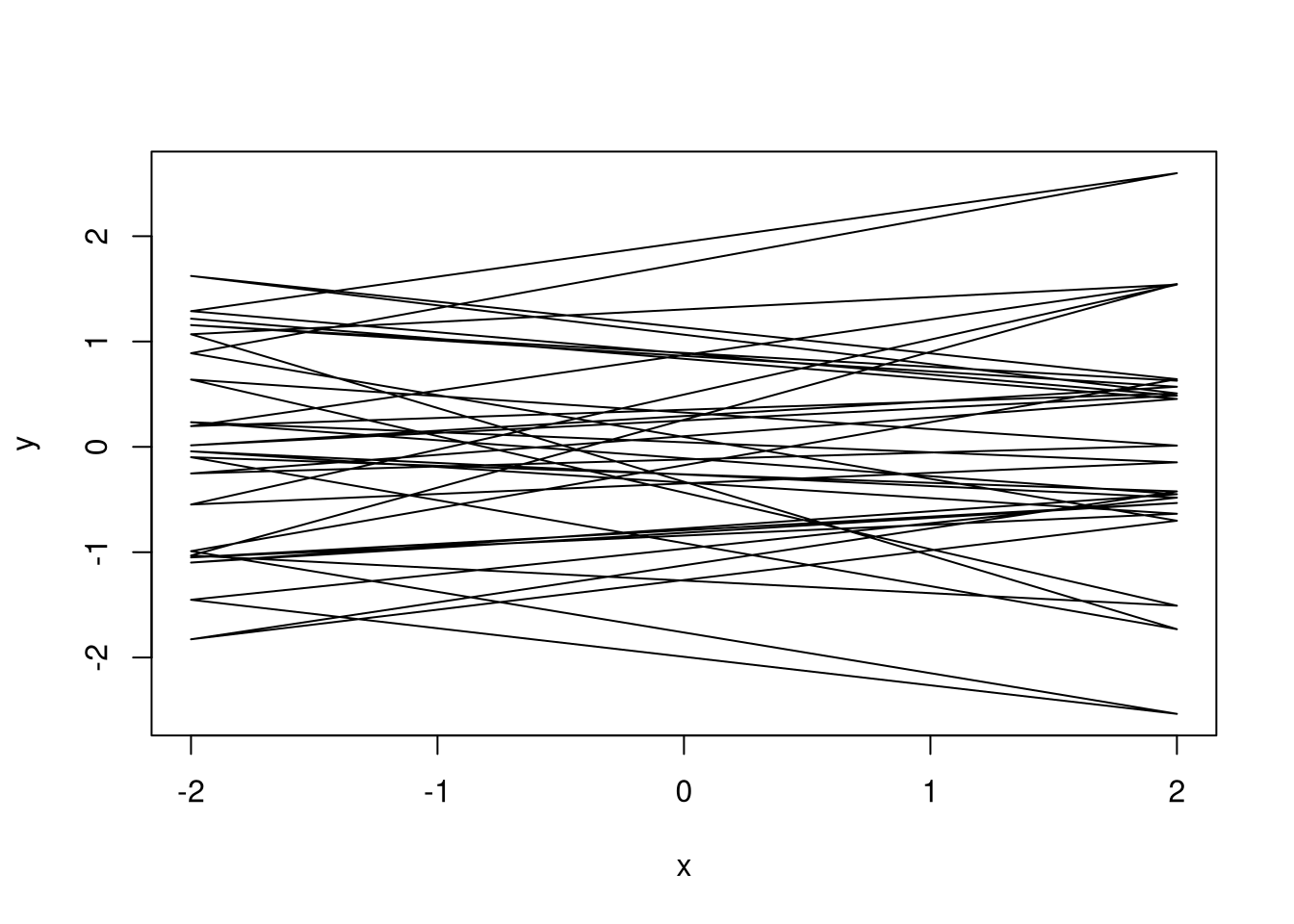

## NULL

3.2.4 Paths

Interest: Area on Weight

Paths

Area -> Avgfood -> Weight
Area -> Avgfood -> Groupsize -> Weight

Avgfood and Groupsize are pipes between Area and Weight. There are no backdoors or colliders.

3.2.5 Interpretation

Would increasing the area available to each fox make it heavier (healthier)?

bArea has a mean of 0.02, with compatibility intervals around 0. Therefore the model does not indicate a total causal influence of area on the weight.

precis(m1)

##            mean    sd  5.5% 94.5%
## a     -0.000001 0.044 -0.07  0.07
## bArea  0.018844 0.091 -0.13  0.16
## sigma  0.995497 0.065  0.89  1.10

post <- extract.samples(m1)
s <- sim(m1, data = list(scale_area = c(-2, 2)), post = post)

ggplot(data.table(s), aes(V1)) +
    stat_halfeye(.width = .89)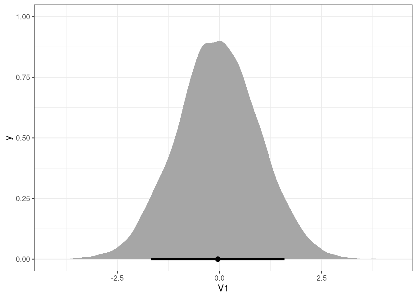

3.3 Question 2

Now infer the causal impact of adding food to a territory. Would this make foxes heavier? Which covariates do you need to adjust for to estimate the total causal influence of food?

3.3.1 Paths

Interest: Food on weight

Paths:

Food -> Weight
Food -> Groupsize -> Weight

Groupsize is a pipe between Area and Weight. There are no backdoors or colliders.

3.3.2 Model

foxes$scale_avgfood <- scale(foxes$avgfood)

m2 <- quap(
    alist(
        scale_weight ~ dnorm(mu, sigma),
        mu <- a + bFood * scale_avgfood,
        a ~ dnorm(0, 0.05),
        bFood ~ dnorm(0, 0.5),
        sigma ~ dunif(0, 50)
    ), 
    data = foxes
)

precis(m2)

##             mean    sd  5.5% 94.5%
## a      0.0000018 0.044 -0.07  0.07
## bFood -0.0241757 0.091 -0.17  0.12
## sigma  0.9953723 0.065  0.89  1.10

post <- extract.samples(m2)
s <- sim(m2, data = list(scale_avgfood = c(-2, 2)), post = post)

ggplot(data.table(s), aes(V1)) +
    stat_halfeye(.width = .89)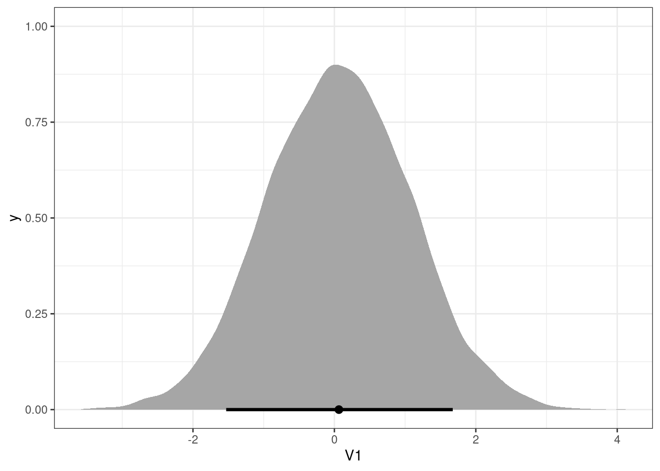

3.3.3 Interpretation

Would this make foxes heavier? Which covariates do you need to adjust for to estimate the total causal influence of food?

bFood has a mean of -0.02, with compatibility intervals around 0. The model does not indicate a total causal influence of area on the weight. No covariates are needed to estiamte the total causal influence of food because there are no backdoors or colliders.

3.4 Question 3

Now infer the causal impact of group size. Which covariates do you need to adjust for? Looking at the posterior distribution of the resulting model, what do you think explains these data? That is, can you explain the estimates for all three problems? How do they go together?

3.4.1 Paths

Interest: Group size on weight

Paths:

Groupsize -> Weight
Groupsize <- Avgfood -> Weight

Avgfood is a collider between Groupsize and Weight. There is a backdoor on Groupsize and the path is closed.

foxes$scale_groupsize <- scale(foxes$groupsize)

m3 <- quap(
    alist(
        scale_weight ~ dnorm(mu, sigma),
        mu <- a + bGroupsize * scale_groupsize + bFood * scale_avgfood,
        a ~ dnorm(0, 0.05),
        bGroupsize ~ dnorm(0, 0.5),
        bFood ~ dnorm(0, 0.5),
        sigma ~ dunif(0, 50)
    ), 
    data = foxes
)

precis(m3)

##                   mean    sd   5.5%  94.5%
## a           0.00000062 0.043 -0.069  0.069
## bGroupsize -0.57250071 0.180 -0.860 -0.285
## bFood       0.47624205 0.180  0.189  0.763
## sigma       0.94590281 0.062  0.846  1.046

DT <- melt(data.table(extract.samples(m3))[, .(bGroupsize, bFood)])

## Warning in melt.data.table(data.table(extract.samples(m3))[, .(bGroupsize, :
## id.vars and measure.vars are internally guessed when both are 'NULL'. All
## non-numeric/integer/logical type columns are considered id.vars, which in this
## case are columns []. Consider providing at least one of 'id' or 'measure' vars
## in future.

ggplot(DT) + 
    geom_density(aes(value, fill = variable), alpha = 0.6) + 
    theme_bw() + scale_fill_viridis_d(begin = 0.3, end = 0.8)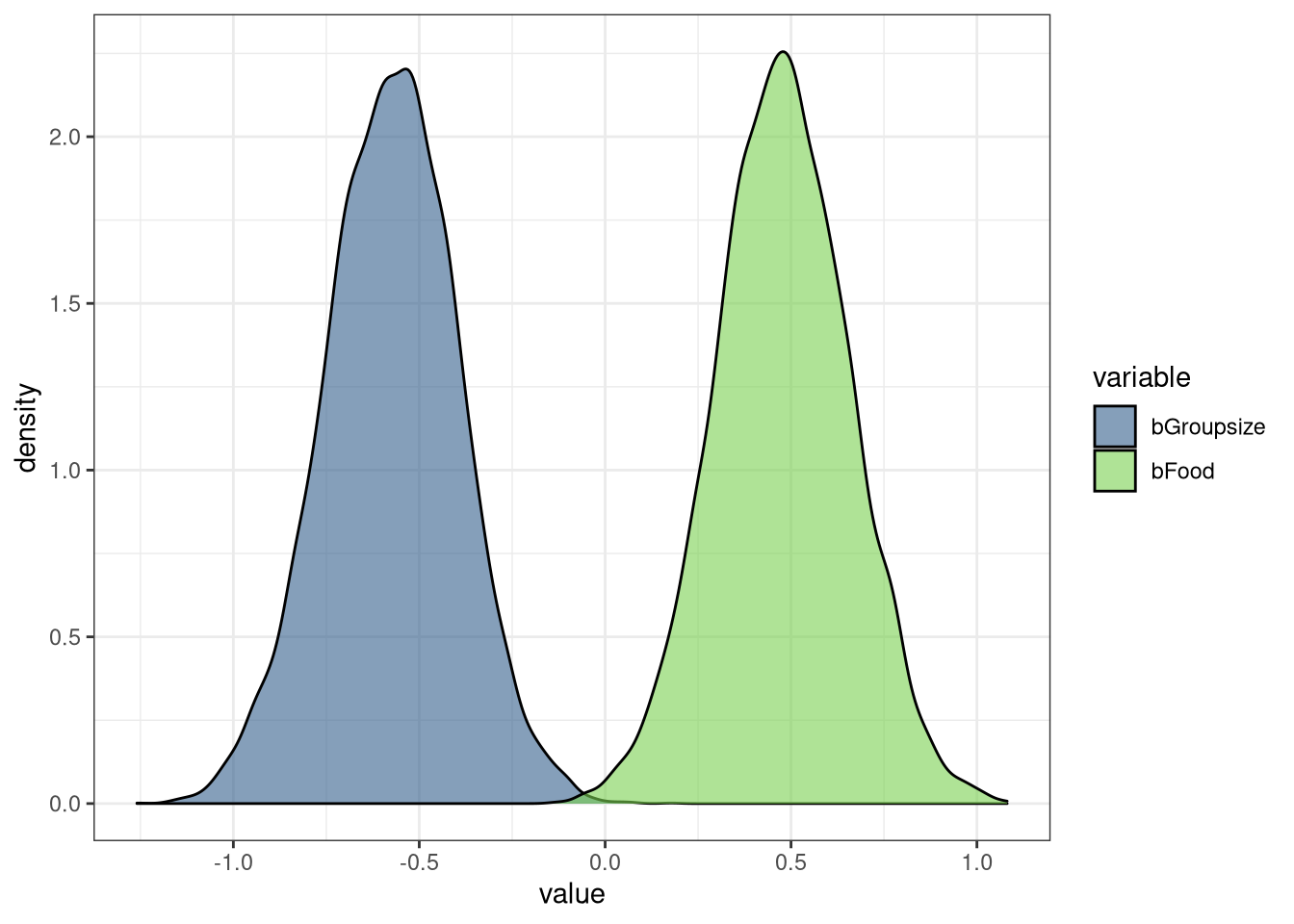

3.4.2 Interpretation

Which covariates do you need to adjust for? Looking at the posterior distribution of the resulting model, what do you think explains these data? That is, can you explain the estimates for all three problems? How do they go together?

The Avgfood covariate needs to be included since it is a collider between Groupsize and Weight. The mean and compatibility intervals of bFood are positive, while the mean and compatibility intervals of bGroupsize are negative. This indicates food’s positive relationship with weight could be buffered or interacting with the negative relationship of group size. Increased food leads to increased body weight, but more food also results in larger groups, which decreases the food availability.

2 Week 2

4 Week 4