6 Week 6

2021-09-06 [updated: 2022-01-26]

6.1 Question 1

The data in data(NWOGrants) are outcomes for scientific funding applications for the Netherlands Organization for Scientific Research (NWO) from 2010–2012 (see van der Lee and Ellemers doi:10.1073/pnas.1510159112). These data have a very similar structure to the UCBAdmit data discussed in Chapter 11. I want you to consider a similar question: What are the total and indirect causal effects of gender on grant awards? Consider a mediation path (a pipe) through dis- cipline. Draw the corresponding DAG and then use one or more binomial GLMs to answer the question.

6.1.1 Data

DT <- data_grants()

precis(DT)

##                   mean     sd 5.5% 94.5%     histogram
## discipline         NaN     NA   NA    NA              
## gender             NaN     NA   NA    NA              
## applications     156.8 119.52 37.0   410     ▅▇▅▅▃▂▁▁▃
## awards            25.9  15.95  8.5    48 ▂▅▅▇▂▇▅▂▁▅▁▁▂
## index_gender       1.5   0.51  1.0     2    ▇▁▁▁▁▁▁▁▁▇
## index_discipline   5.0   2.66  1.0     9      ▇▃▃▃▃▃▃▃

summary(DT)

##                discipline gender  applications     awards    index_gender
##  Chemical sciences  :2    f:9    Min.   :  9   Min.   : 2   Min.   :1.0  
##  Earth/life sciences:2    m:9    1st Qu.: 70   1st Qu.:14   1st Qu.:1.0  
##  Humanities         :2           Median :130   Median :24   Median :1.5  
##  Interdisciplinary  :2           Mean   :157   Mean   :26   Mean   :1.5  
##  Medical sciences   :2           3rd Qu.:220   3rd Qu.:33   3rd Qu.:2.0  
##  Physical sciences  :2           Max.   :425   Max.   :65   Max.   :2.0  
##  (Other)            :6                                                   
##  index_discipline
##  Min.   :1       
##  1st Qu.:3       
##  Median :5       
##  Mean   :5       
##  3rd Qu.:7       
##  Max.   :9       
##

Discipline: factor with 9 levels
Gender: factor with 2 levels in this data (…)
Applications: count
Awards: count

q1_data <- c(
    as.list(DT[, .(awards, applications, index_gender, index_discipline)]),
    N = DT[, .N],
    N_gender = DT[, uniqueN(index_gender)],
    N_discipline = DT[, uniqueN(index_discipline)]
)

6.1.2 DAG

dag <- dagify(
    awards ~ index_gender + index_discipline,
    index_discipline ~ index_gender,
    exposure = 'index_gender',
    outcome = 'awards'
)

dag_plot(dag)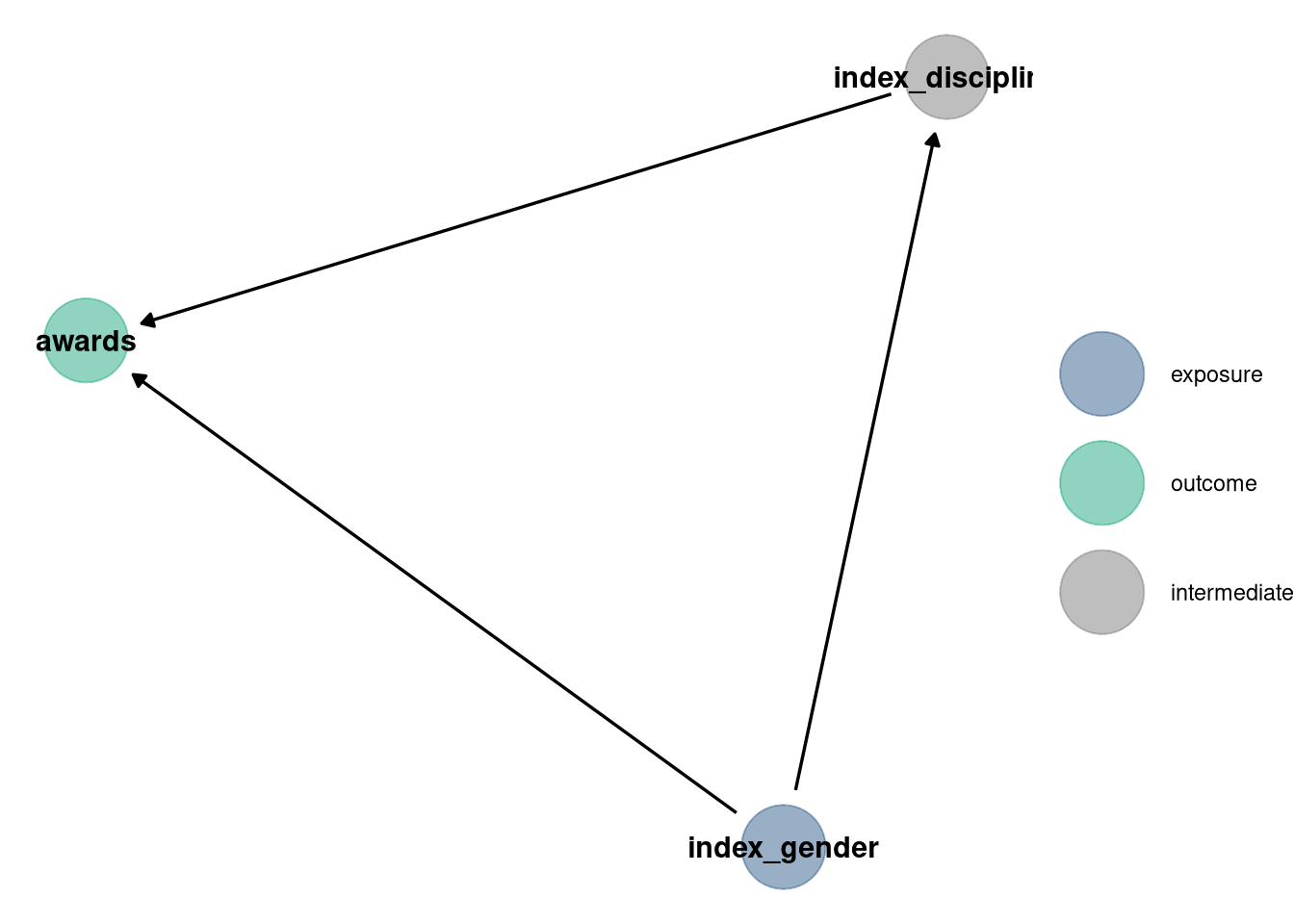

6.1.3 Priors

writeLines(readLines(tar_read(stan_b_file_w06_q1_prior)))

## data {
##   int<lower=0> N;
##   int<lower=0> N_gender;
##   int<lower=0> N_discipline;
## }
## parameters{
##   real alpha;
##   vector[N_gender] beta_gender;
##   vector[N_discipline] beta_discipline;
##   real<lower=0> sigma;
##   real<lower=0,upper=1> theta;
## }
## model{
##   alpha ~ normal(0, 0.2);
##   beta_gender ~ normal(0, 0.25);
##   beta_discipline ~ normal(0, 0.25);
##   sigma ~ exponential(1);
##   theta ~ beta(1, 1);
## }

q1_prior_draws <- tar_read(stan_b_mcmc_w06_q1_prior)$draws()

mcmc_areas(q1_prior_draws, regex_pars = 'theta')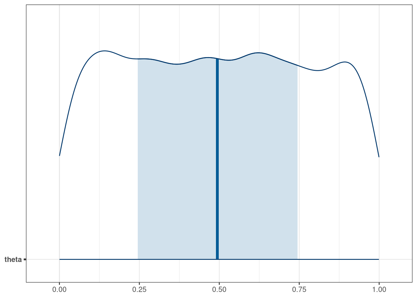

mcmc_areas(q1_prior_draws, regex_pars = 'sigma')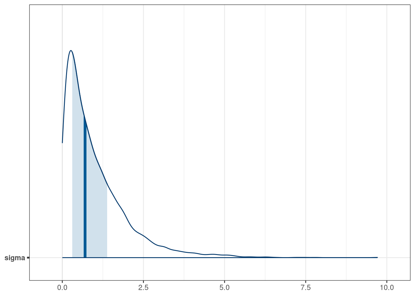

mcmc_areas(q1_prior_draws, regex_pars = 'beta_gender')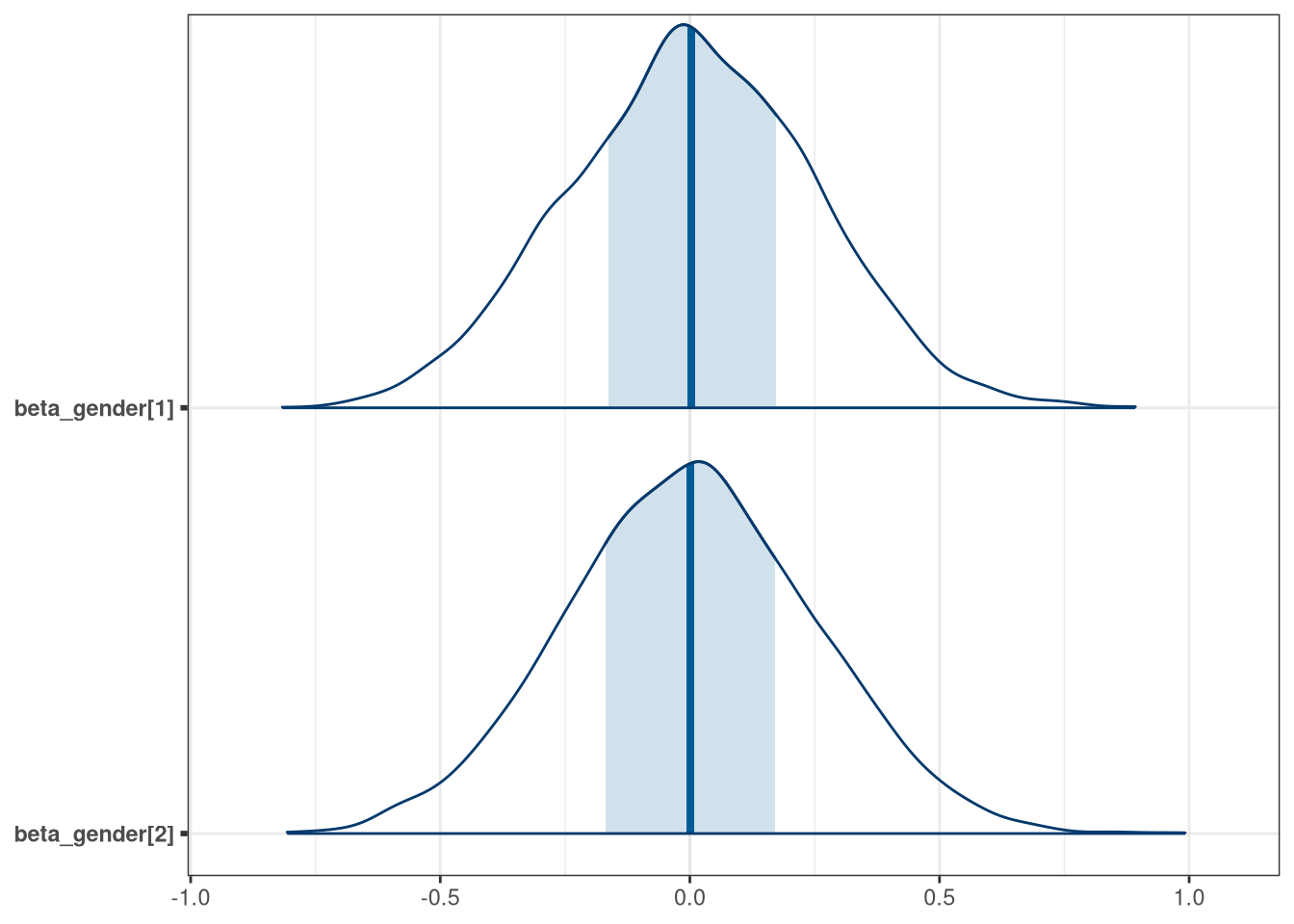

mcmc_areas(q1_prior_draws, regex_pars = 'beta_discipline')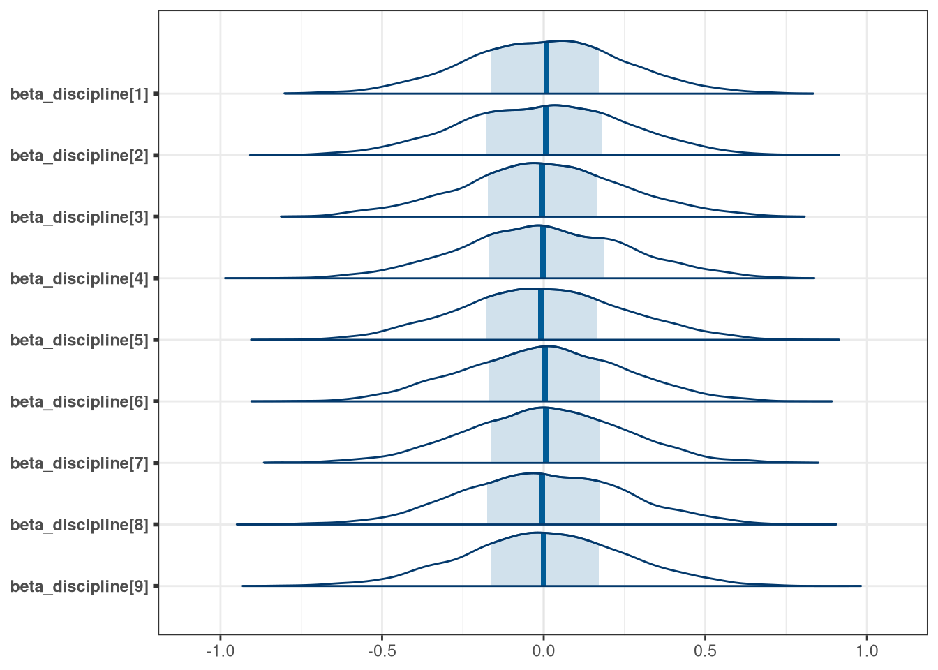

6.1.4 Model

writeLines(readLines(tar_read(stan_b_file_w06_q1)))

## data {
##   int<lower=0> N;
##   int<lower=0> N_gender;
##   int awards[N];
##   int applications [N];
##   int index_gender[N];
## }
## parameters{
##   vector[N_gender] alpha;
## }
## model{
##   vector[N] p;
##   alpha ~ normal(-1, 1);
## 
##   p = inv_logit(alpha[index_gender]);
##   awards ~ binomial(applications, p);
## }

q1_draws <- tar_read(stan_b_mcmc_w06_q1)$draws()

mcmc_areas(q1_draws, regex_pars = 'alpha')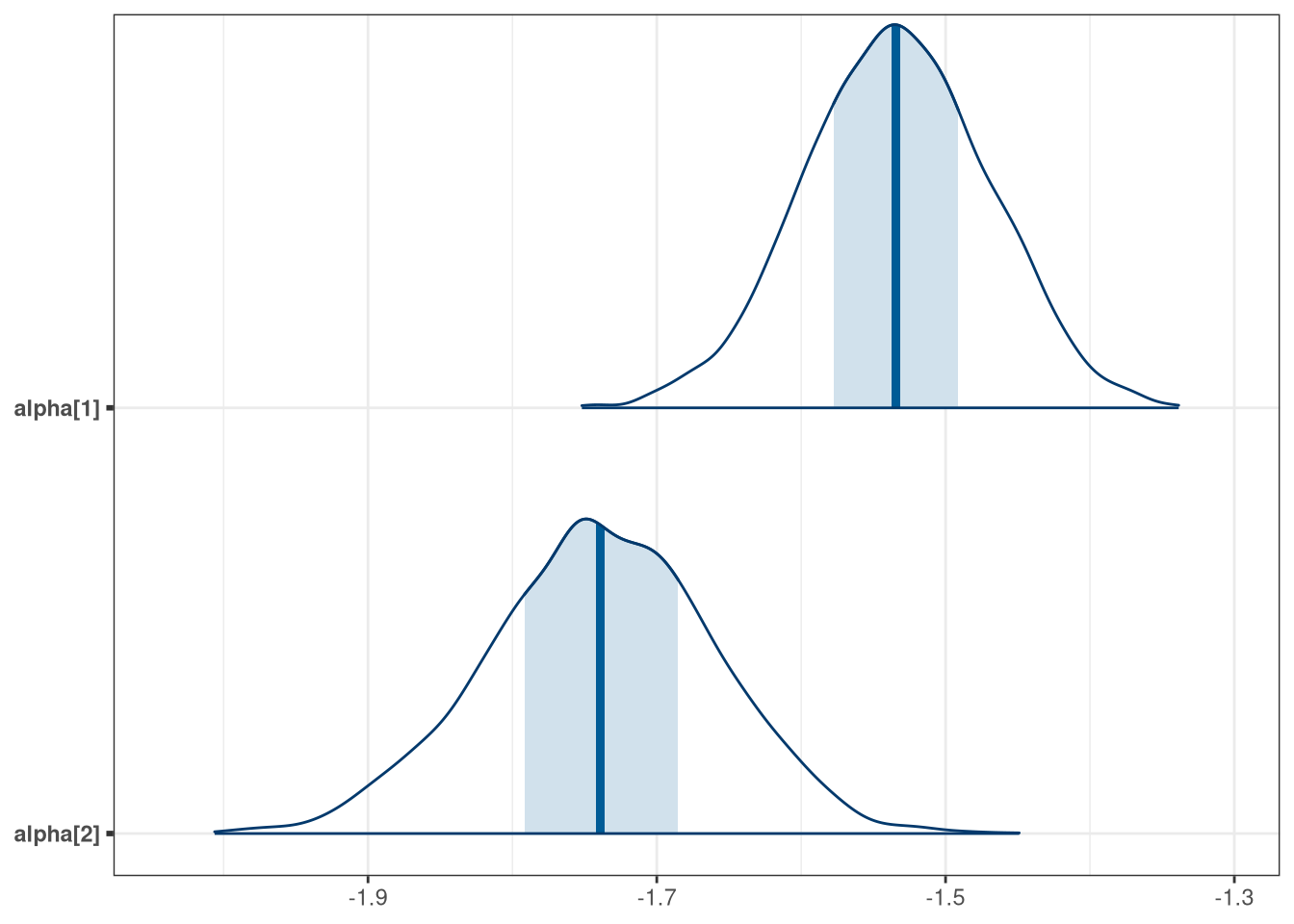

q1_draws$dif_alpha <- (inv.logit(q1_draws$`alpha[1]`) -
    inv.logit(q1_draws$`alpha[2]`)) * 100
mcmc_areas(q1_draws, regex_pars = 'dif_alpha')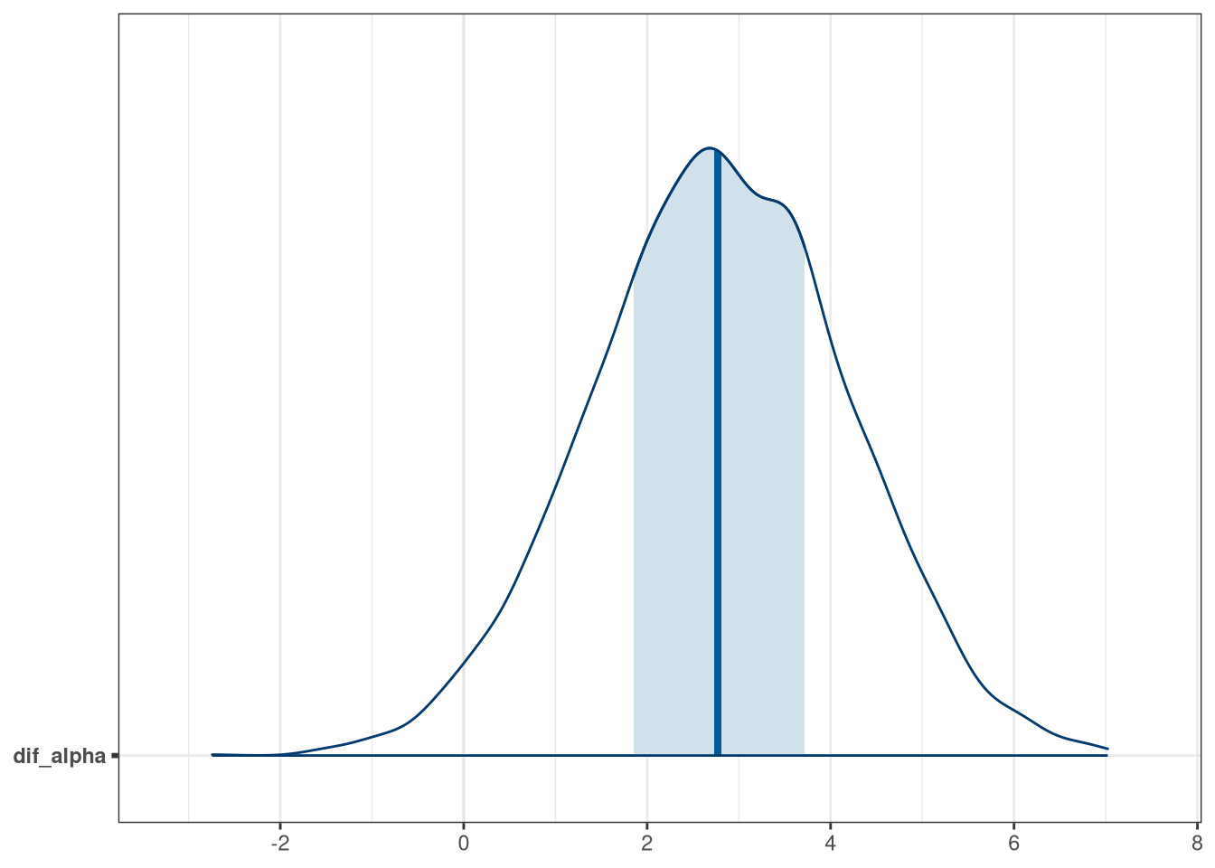

With discipline

writeLines(readLines(tar_read(stan_b_file_w06_q1_discipline)))

## data {
##   int<lower=0> N;
##   int<lower=0> N_gender;
##   int<lower=0> N_discipline;
##   int awards[N];
##   int applications [N];
##   int index_gender[N];
##   int index_discipline[N];
## }
## parameters{
##   vector[N_gender] alpha;
##   vector[N_discipline] beta;
## }
## model{
##   vector[N] p;
##   alpha ~ normal(-1, 1);
##   beta ~ normal(0, 0.25);
## 
##   p = inv_logit(alpha[index_gender] + beta[index_discipline]);
##   awards ~ binomial(applications, p);
## }

q1_discipline_draws <- tar_read(stan_b_mcmc_w06_q1_discipline)$draws()

mcmc_areas(q1_discipline_draws, regex_pars = 'alpha')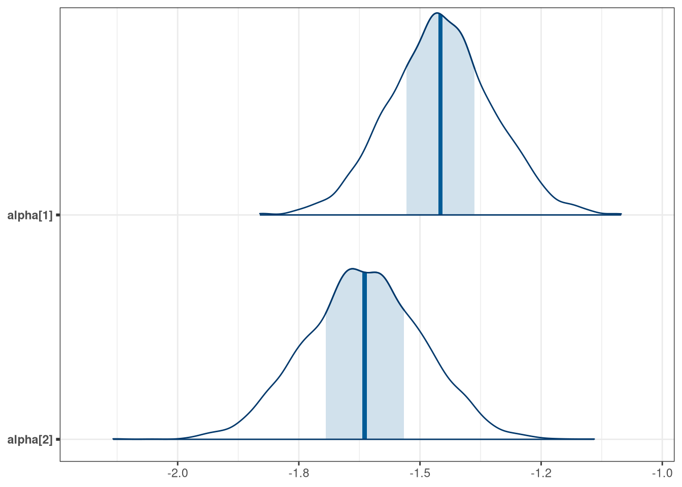

mcmc_areas(q1_discipline_draws, regex_pars = 'beta')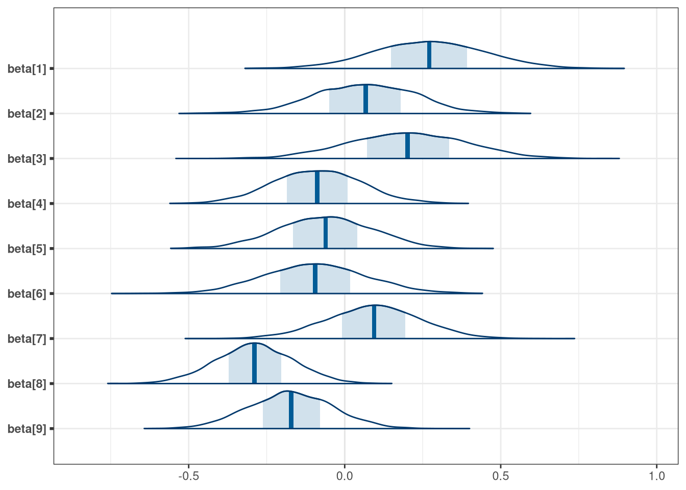

# Need to account for base rates to look at absolute rate
# q1_draws$dif_alpha <- (inv.logit(q1_draws$`alpha[1]`) -
#   inv.logit(q1_draws$`alpha[2]`)) * 100
# mcmc_areas(q1_draws, regex_pars = 'dif_alpha')

# We can look at relative rates though
q1_discipline_draws$dif_alpha_rel <- q1_discipline_draws$`alpha[1]` - q1_discipline_draws$`alpha[2]`
mcmc_areas(q1_discipline_draws, regex_pars = 'dif_alpha_rel')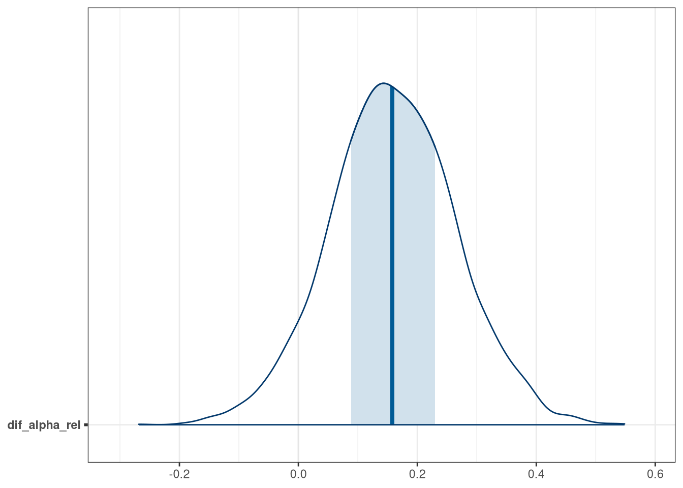

What is your causal interpretation? If NWO’s goal is to equalize rates of funding between the genders, what type of intervention would be most effective?

Investigate departmental levels, since once this is included the relative differences are small.

5 Week 5

7 Week 7