9 Week 9
2021-09-14 [updated: 2022-01-26]
9.1 Question 1
Revisit the Bangladesh fertility data, data(bangladesh). Fit a model with both varying intercepts by district_id and varying slopes of urban (as a 0/1 indicator variable) by district_id. You are still predicting use.contraception. Inspect the correlation between the intercepts and slopes. Can you interpret this correlation, in terms of what it tells you about the pattern of contraceptive use in the sample? It might help to plot the varying effect estimates for both the intercepts and slopes, by district. Then you can visualize the correlation and maybe more easily think through what it means to have a particular correlation. Plotting predicted proportion of women using contraception, in each district, with urban women on one axis and rural on the other, might also help.
precis(DT)## mean sd 5.5% 94.5% histogram
## case NaN NA NA NA
## response 4.20 1.91 1 7 ▃▂▁▃▁▇▁▅▁▅▁▅
## order 16.50 9.29 2 31 ▇▅▇▇▅▇▂
## id NaN NA NA NA
## age 37.49 14.23 18 61 ▂▇▅▇▅▇▅▅▃▅▂▁▁
## male 0.57 0.49 0 1 ▅▁▁▁▁▁▁▁▁▇
## edu NaN NA NA NA
## action 0.43 0.50 0 1 ▇▁▁▁▁▁▁▁▁▅
## intention 0.47 0.50 0 1 ▇▁▁▁▁▁▁▁▁▇
## contact 0.20 0.40 0 1 ▇▁▁▁▁▁▁▁▁▂
## story NaN NA NA NA
## action2 0.63 0.48 0 1 ▃▁▁▁▁▁▁▁▁▇
## education 5.73 1.35 3 8 ▁▁▁▁▁▂▁▅▁▇▁▂▁▂
## individual 166.00 95.56 19 313 ▇▇▇▇▇▇▅
writeLines(readLines(tar_read(stan_e_file_w09_model_q1)))## data {
## // Integers for number of rows, and number of districts
## int<lower=0> N;
## int<lower=0> N_district;
##
## // District, contraception and urban, expecting integers of length N
## int district[N];
## int contraception[N];
## int urban[N];
## }
## parameters {
## // Alpha and beta urban vectors matching length of number of districts
## vector[N_district] alpha;
##
## // Beta urban vector matching length of number of districts
## vector[N_district] beta;
##
## // Hyper parameter alpha bar, beta bar
## real alpha_bar;
## real beta_bar;
##
## // Correlation matrix, sigma
## // 2 represents the number of predictors
## corr_matrix[2] Rho;
## vector<lower=0>[2] sigma;
## }
## model {
## // p vector matching length of number of districts
## vector[N] p;
##
## // Hyper priors: alpha bar, beta urban bar, sigma and Rho
## alpha_bar ~ normal(0, 1);
## beta_bar ~ normal(0, 0.5);
## sigma ~ exponential(1);
## Rho ~ lkj_corr(2);
##
## // Multivariate normal
## {
## vector[2] YY[N_district];
## vector[2] MU;
## MU = [alpha_bar, beta_bar]';
## for (j in 1:N_district) {
## YY[j] = [alpha[j], beta[j]]';
## }
## YY ~ multi_normal(MU, quad_form_diag(Rho, sigma));
## }
##
## // For each for in data, alpha and beta for that row's district
## for (i in 1:N) {
## p[i] = inv_logit(alpha[district[i]] + beta[district[i]] * urban[i]);
## }
##
## // Contraception if distributed with bernoulli, p
## contraception ~ bernoulli(p);
## }
model_q1_draws <- tar_read(stan_e_mcmc_w09_model_q1)$draws()

mcmc_areas(model_q1_draws, regex_pars = 'alpha')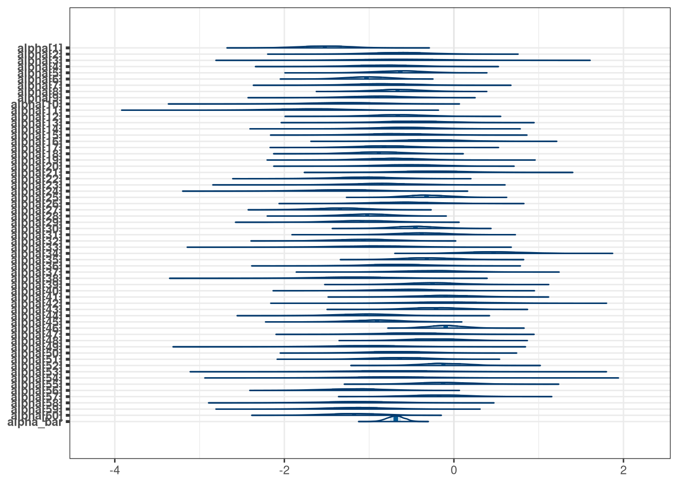
mcmc_areas(model_q1_draws, regex_pars = 'beta')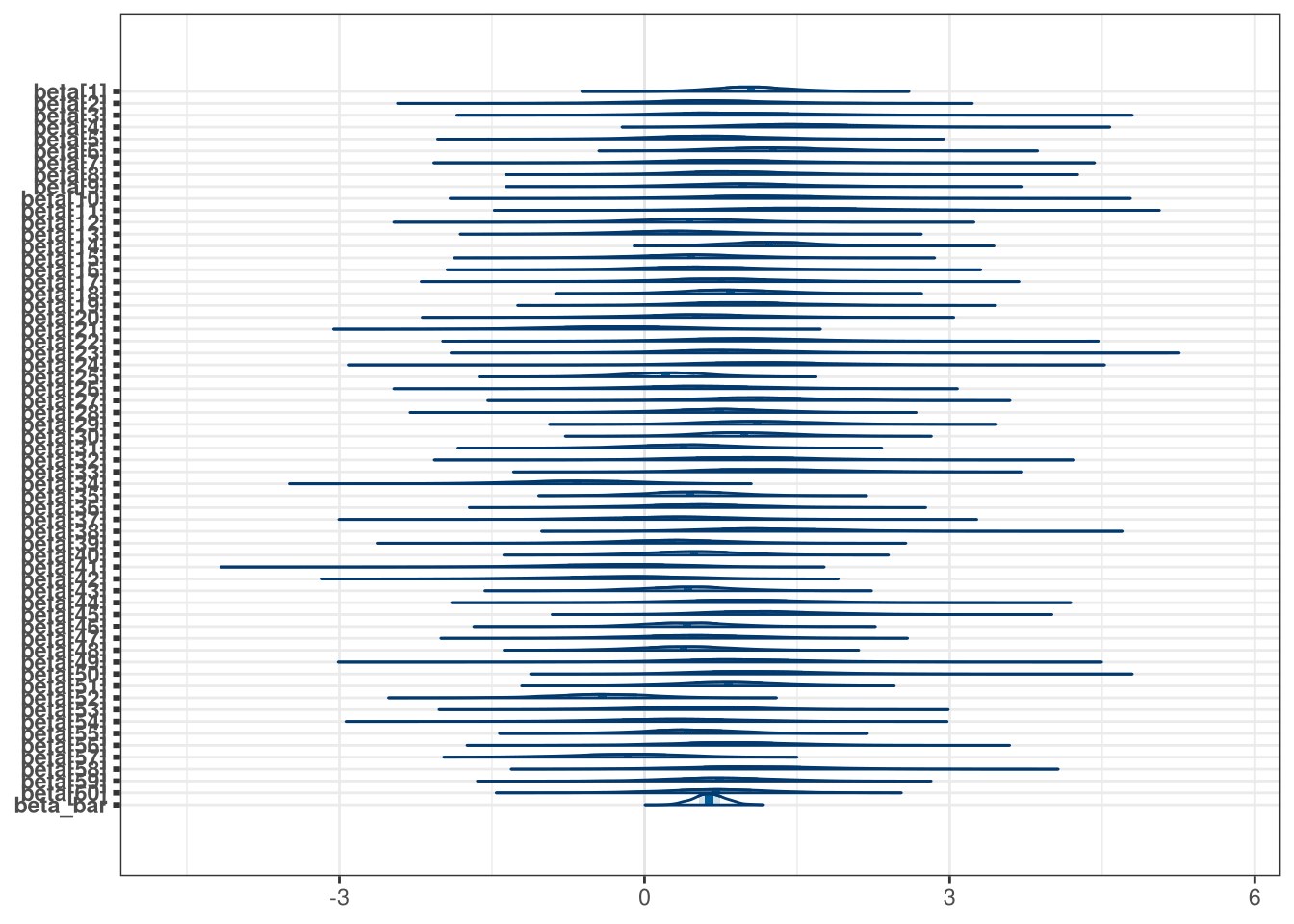
mcmc_areas(model_q1_draws, regex_pars = 'bar')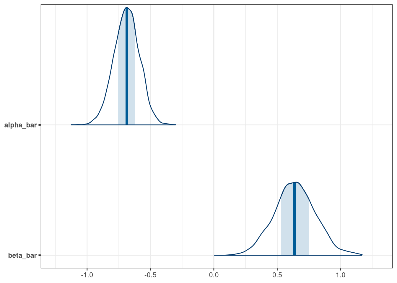
mcmc_areas(model_q1_draws, regex_pars = 'Rho')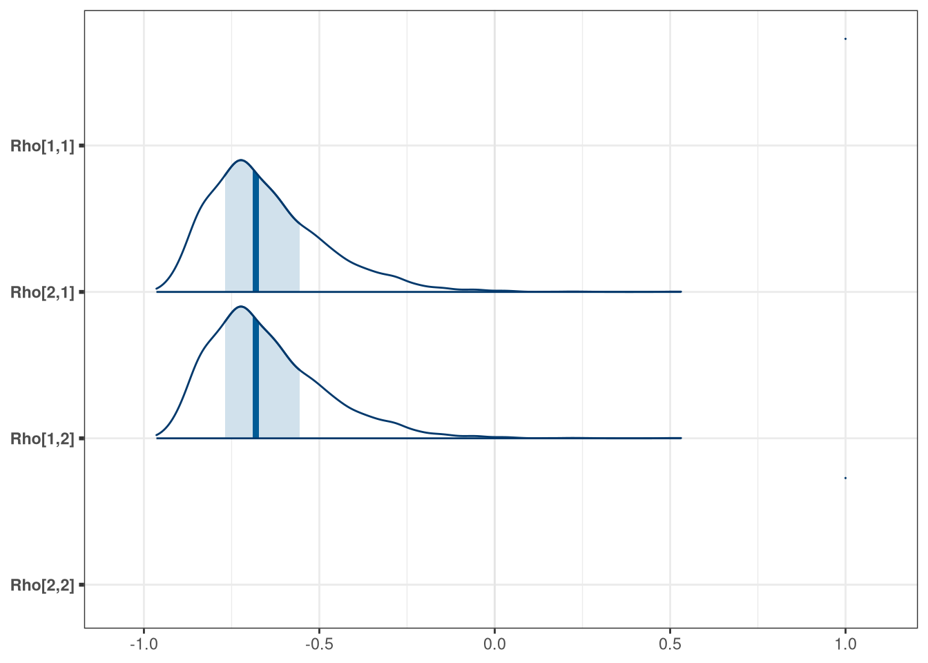
setDT(model_q1_draws)

precis(model_q1_draws[, .SD, .SDcols = patterns('*bar')])
## mean sd 5.5% 94.5% histogram
## alpha_bar -0.69 0.10 -0.85 -0.53 ▁▁▁▂▇▇▃▁▁
## beta_bar 0.64 0.16 0.38 0.90 ▁▁▁▂▃▇▇▅▃▁▁▁
precis(model_q1_draws[, .SD, .SDcols = patterns('Rho|sigma')], depth = 3)## mean sd 5.5% 94.5% histogram
## Rho[1,1] 1.00 0.000 1.00 1.00 ▇
## Rho[2,1] -0.65 0.168 -0.86 -0.34 ▂▇▃▁▁▁▁▁
## Rho[1,2] -0.65 0.168 -0.86 -0.34 ▂▇▃▁▁▁▁▁
## Rho[2,2] 1.00 0.000 1.00 1.00 ▇
## sigma[1] 0.57 0.096 0.43 0.74 ▁▁▁▂▅▇▇▇▃▂▁▁▁▁
## sigma[2] 0.77 0.207 0.46 1.10 ▁▁▃▇▅▂▁▁▁
mcmc_hex(model_q1_draws, regex_pars = '*bar')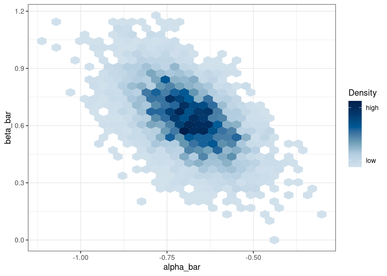
9.2 Question 2
Now consider the predictor variables age.centered and living.children, also contained in data(bangladesh). Suppose that age influences contraceptive use (changing attitudes) and number of children (older people have had more time to have kids). Number of children may also directly influence contraceptive use. Draw a DAG that reflects these hypothetical relationships. Then build models needed to evaluate the DAG. You will need at least two models. Retain district and urban, as in Problem 1. What do you conclude about the causal influence of age and children?
dag <- dagify(
  contraceptive_use ~ age + number_children,
  number_children ~ age,
  exposure = 'age',
  outcome = 'contraceptive_use'
)

dag_plot(dag)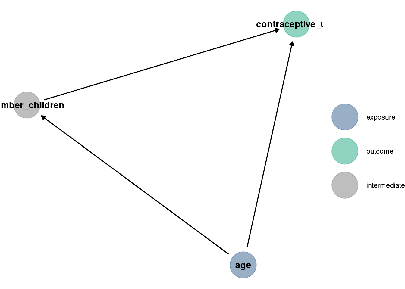
adjustmentSets(dag, exposure = 'age', outcome = 'contraceptive_use', effect = 'total')## {}
adjustmentSets(dag, exposure = 'age', outcome = 'contraceptive_use', effect = 'direct')## { number_children }
writeLines(readLines(tar_read(stan_e_file_w09_model_q2_a)))## data {
## // Integers for number of rows, and number of districts
## int<lower=0> N;
## int<lower=0> N_district;
##
## // District, contraception and urban, expecting integers of length N
## int district[N];
## int contraception[N];
## int urban[N];
##
## // Also scale_age
## real scale_age[N];
## }
## parameters {
## // Alpha and beta urban vectors matching length of number of districts
## vector[N_district] alpha;
##
## // Beta urban vector matching length of number of districts
## vector[N_district] beta;
##
## // Hyper parameter alpha bar, beta bar
## real alpha_bar;
## real beta_bar;
##
## // scale_age
## real beta_scale_age;
##
## // Correlation matrix, sigma
## // 2 represents the number of predictors
## corr_matrix[2] Rho;
## vector<lower=0>[2] sigma;
## }
## model {
## // p vector matching length of number of districts
## vector[N] p;
##
## // Hyper priors: alpha bar, beta urban bar, sigma and Rho
## alpha_bar ~ normal(0, 1);
## beta_bar ~ normal(0, 0.5);
## sigma ~ exponential(1);
## Rho ~ lkj_corr(2);
##
## // Multivariate normal
## {
## vector[2] YY[N_district];
## vector[2] MU;
## MU = [alpha_bar, beta_bar]';
## for (j in 1:N_district) {
## YY[j] = [alpha[j], beta[j]]';
## }
## YY ~ multi_normal(MU, quad_form_diag(Rho, sigma));
## }
##
## // Beta scale_age prior
## beta_scale_age ~ normal(0, 1.5);
##
## // For each for in data, alpha and beta for that row's district
## for (i in 1:N) {
## p[i] = inv_logit(alpha[district[i]] + beta[district[i]] * urban[i] + beta_scale_age * scale_age[i]);
## }
##
## // Contraception if distributed with bernoulli, p
## contraception ~ bernoulli(p);
## }
model_q2_a_draws <- tar_read(stan_e_mcmc_w09_model_q2_a)$draws()
setDT(model_q2_a_draws)
writeLines(readLines(tar_read(stan_e_file_w09_model_q2_b)))## data {
## // Integers for number of rows, and number of districts
## int<lower=0> N;
## int<lower=0> N_district;
##
## // District, contraception and urban, expecting integers of length N
## int district[N];
## int contraception[N];
## int urban[N];
##
## // Also scale_age and n_children
## real scale_age[N];
## int n_children[N];
## }
## parameters {
## // Alpha and beta urban vectors matching length of number of districts
## vector[N_district] alpha;
##
## // Beta urban vector matching length of number of districts
## vector[N_district] beta;
##
## // Hyper parameter alpha bar, beta bar
## real alpha_bar;
## real beta_bar;
##
## // scale_age and n_children
## real beta_scale_age;
## real beta_children;
##
## // Correlation matrix, sigma
## // 2 represents the number of predictors
## corr_matrix[2] Rho;
## vector<lower=0>[2] sigma;
## }
## model {
## // p vector matching length of number of districts
## vector[N] p;
##
## // Hyper priors: alpha bar, beta urban bar, sigma and Rho
## alpha_bar ~ normal(0, 1);
## beta_bar ~ normal(0, 0.5);
## sigma ~ exponential(1);
## Rho ~ lkj_corr(2);
##
## // Multivariate normal
## {
## vector[2] YY[N_district];
## vector[2] MU;
## MU = [alpha_bar, beta_bar]';
## for (j in 1:N_district) {
## YY[j] = [alpha[j], beta[j]]';
## }
## YY ~ multi_normal(MU, quad_form_diag(Rho, sigma));
## }
##
## // Beta scale_age prior
## beta_scale_age ~ normal(0, 1.5);
## beta_children ~ normal(0, 1.5);
##
## // For each for in data, alpha and beta for that row's district
## for (i in 1:N) {
## p[i] = inv_logit(alpha[district[i]] + beta[district[i]] * urban[i] + beta_scale_age * scale_age[i] + beta_children * n_children[i]);
## }
##
## // Contraception if distributed with bernoulli, p
## contraception ~ bernoulli(p);
## }
model_q2_b_draws <- tar_read(stan_e_mcmc_w09_model_q2_b)$draws()
setDT(model_q2_b_draws)
precis(model_q2_a_draws[, .SD, .SDcols = patterns('beta')])## 60 vector or matrix parameters hidden. Use depth=2 to show them.## mean sd 5.5% 94.5% histogram
## beta_bar 0.643 0.16 0.3844 0.90 ▁▁▁▁▃▇▇▅▃▁▁▁▁▁
## beta_scale_age 0.084 0.05 0.0057 0.16 ▁▁▃▇▅▂▁▁
precis(model_q2_b_draws[, .SD, .SDcols = patterns('beta')])## 60 vector or matrix parameters hidden. Use depth=2 to show them.## mean sd 5.5% 94.5% histogram
## beta_bar 0.68 0.163 0.42 0.93 ▁▁▁▁▃▅▇▇▃▂▁▁▁
## beta_scale_age -0.26 0.071 -0.38 -0.15 ▁▁▁▁▂▅▇▇▃▁▁▁
## beta_children 0.41 0.060 0.32 0.51 ▁▁▃▇▇▃▁▁▁9.3 Question 3
Modify any models from Problem 2 that contained that children variable and model the variable now as a monotonic ordered category, like education from the week we did ordered categories. Education in that example had 8 categories. Children here will have fewer (no one in the sample had 8 children). So modify the code appropriately. What do you conclude about the causal influence of each additional child on use of contraception?
writeLines(readLines(tar_read(stan_e_file_w09_model_q3)))## data {
## // Integers for number of rows, and number of districts
## int<lower=0> N;
## int<lower=0> N_district;
##
## // K categories
## int K;
## vector[K] alpha_k;
##
## // District, contraception and urban, expecting integers of length N
## int district[N];
## int contraception[N];
## int urban[N];
##
## // Also scale_age, n_children
## real scale_age[N];
## int n_children[N];
## }
## parameters {
## // Alpha and beta urban vectors matching length of number of districts
## vector[N_district] alpha;
##
## // Beta urban vector matching length of number of districts
## vector[N_district] beta;
##
## // Hyper parameter alpha bar, beta bar
## real alpha_bar;
## real beta_bar;
##
## // scale_age and n_children
## real beta_scale_age;
## real beta_children;
##
## // Correlation matrix, sigma
## // 2 represents the number of predictors
## corr_matrix[2] Rho;
## vector<lower=0>[2] sigma;
##
## simplex[3] delta;
## }
## model {
## // p vector matching length of number of districts
## vector[N] p;
##
## // Hyper priors: alpha bar, beta urban bar, sigma and Rho
## alpha_bar ~ normal(0, 1);
## beta_bar ~ normal(0, 0.5);
## sigma ~ exponential(1);
## Rho ~ lkj_corr(2);
##
## //
## vector[K] delta_shell;
## delta ~ dirichlet(alpha_k);
## delta_shell = append_row(0, delta);
##
## // Multivariate normal
## {
## vector[2] YY[N_district];
## vector[2] MU;
## MU = [alpha_bar, beta_bar]';
## for (j in 1:N_district) {
## YY[j] = [alpha[j], beta[j]]';
## }
## YY ~ multi_normal(MU, quad_form_diag(Rho, sigma));
## }
##
## // Beta scale_age prior
## beta_scale_age ~ normal(0, 1.5);
## beta_children ~ normal(0, 1.5);
##
## // For each for in data, alpha and beta for that row's district
## for (i in 1:N) {
## p[i] = inv_logit(alpha[district[i]] + beta[district[i]] * urban[i] + beta_scale_age * scale_age[i] + beta_children * sum(delta_shell[1:n_children[i]]) * n_children[i]);
## }
##
## // Contraception if distributed with bernoulli, p
## contraception ~ bernoulli(p);
## }
model_q3_draws <- tar_read(stan_e_mcmc_w09_model_q3)$draws()
setDT(model_q3_draws)

precis(model_q3_draws[, .SD, .SDcols = patterns('beta')])
## 60 vector or matrix parameters hidden. Use depth=2 to show them.## mean sd 5.5% 94.5% histogram
## beta_bar 0.69 0.160 0.44 0.94 ▁▁▁▁▂▅▇▇▅▂▁▁▁▁
## beta_scale_age -0.29 0.072 -0.40 -0.17 ▁▁▁▁▃▇▇▅▂▁▁▁
## beta_children 0.34 0.046 0.26 0.41 ▁▁▃▇▇▂▁▁
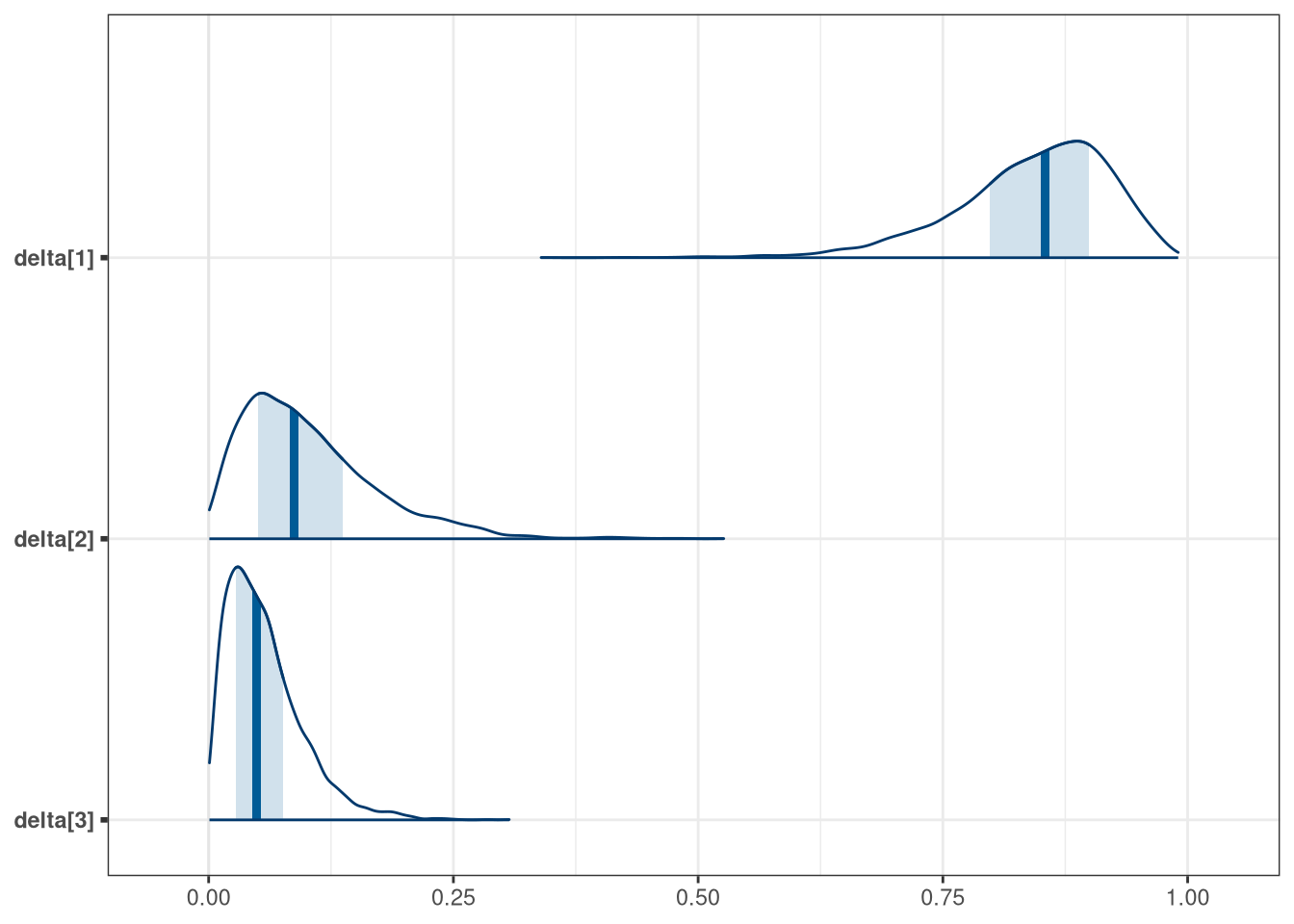
precis(model_q3_draws[, .SD, .SDcols = patterns('delta')], 3)## mean sd 5.5% 94.5% histogram
## delta[1] 0.842 0.079 0.70 0.95 ▁▁▁▁▁▁▁▁▂▃▇▇▅▁
## delta[2] 0.102 0.069 0.02 0.23 ▅▇▅▂▁▁▁▁▁▁▁
## delta[3] 0.056 0.039 0.01 0.13 ▇▅▁▁▁▁▁
mcmc_areas(model_q3_draws, regex_pars = 'delta')