7 Week 7
2021-09-07 [updated: 2022-01-26]
7.0.1 Data
DT <- data_trolley()
precis(DT)
## mean sd 5.5% 94.5% histogram
## case NaN NA NA NA
## response 4.20 1.91 1 7 ▃▂▁▃▁▇▁▅▁▅▁▅
## order 16.50 9.29 2 31 ▇▅▇▇▅▇▂
## id NaN NA NA NA
## age 37.49 14.23 18 61 ▂▇▅▇▅▇▅▅▃▅▂▁▁
## male 0.57 0.49 0 1 ▅▁▁▁▁▁▁▁▁▇
## edu NaN NA NA NA
## action 0.43 0.50 0 1 ▇▁▁▁▁▁▁▁▁▅
## intention 0.47 0.50 0 1 ▇▁▁▁▁▁▁▁▁▇
## contact 0.20 0.40 0 1 ▇▁▁▁▁▁▁▁▁▂
## story NaN NA NA NA
## action2 0.63 0.48 0 1 ▃▁▁▁▁▁▁▁▁▇
## education 5.73 1.35 3 8 ▁▁▁▁▁▂▁▅▁▇▁▂▁▂
## individual 166.00 95.56 19 313 ▇▇▇▇▇▇▅Response: 1-7 integer, “how morally permissible the action to be taken (or not) is”. Categorical, ordered, but distances between categories is not metric or known.
Logit = log-odds, cumulative logit = log-cumulative-odds. Both constrained between 0-1.
Log-cumulative-odds for response 7 will be infinity since log(1/(1-1)) = infinity. Given this, we only need K-1 = 6 intercepts.
7.0.2 Model: ordered categorical outcome
Probability of data: \(R_{i} \sim \text{Ordered-logit}(\phi_{i}, K)\)
Linear model: \(\phi_{i} = 0\)
Prior for each intercept: \(K_{k} \sim \text{Normal}(0, 1.5)\)
writeLines(readLines(tar_read(stan_c_file_w07_model1)))## data {
## int N;
## int K;
## int response[N];
## int action[N];
## int intention[N];
## int contact[N];
## }
## parameters {
## // Cut points are the positions of responses along cumulative odds
## ordered[K] cutpoints;
## real beta_action;
## real beta_intention;
## real beta_contact;
## }
## model {
## vector[N] phi;
##
## for (i in 1:N) {
## phi[i] = beta_action * action[i] + beta_contact * contact[i] + beta_intention * intention[i];
## response[i] ~ ordered_logistic(phi[i], cutpoints);
## }
##
## cutpoints ~ normal(0, 1.5);
## beta_action ~ normal(0, 0.5);
## beta_contact ~ normal(0, 0.5);
## beta_intention ~ normal(0, 0.5);
## }
model1_draws <- tar_read(stan_c_mcmc_w07_model1)$draws()

mcmc_areas(model1_draws, regex_pars = 'beta')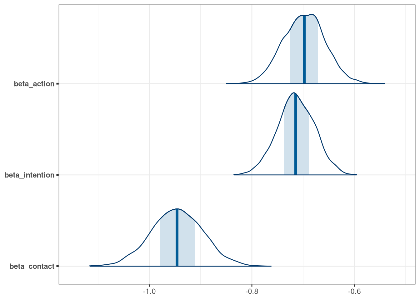
Interactions
writeLines(readLines(tar_read(stan_c_file_w07_model1_interactions)))## data {
## int N;
## int K;
## int response[N];
## int action[N];
## int intention[N];
## int contact[N];
## }
## parameters {
## // Cut points are the positions of responses along cumulative odds
## ordered[K] cutpoints;
## real beta_action;
## real beta_intention;
## real beta_contact;
## real beta_intention_contact;
## real beta_intention_action;
## }
## model {
## vector[N] phi;
##
## for (i in 1:N) {
## phi[i] = beta_action * action[i] + beta_contact * contact[i] + beta_intention * intention[i] + beta_intention_contact * intention[i] * contact[i] + beta_intention_action * intention[i] * action[i]
## ;
## response[i] ~ ordered_logistic(phi[i], cutpoints);
## }
##
## cutpoints ~ normal(0, 1.5);
## beta_action ~ normal(0, 0.5);
## beta_contact ~ normal(0, 0.5);
## beta_intention ~ normal(0, 0.5);
## }
model1_interactions_draws <- tar_read(stan_c_mcmc_w07_model1_interactions)$draws()

mcmc_areas(model1_interactions_draws, regex_pars = 'beta')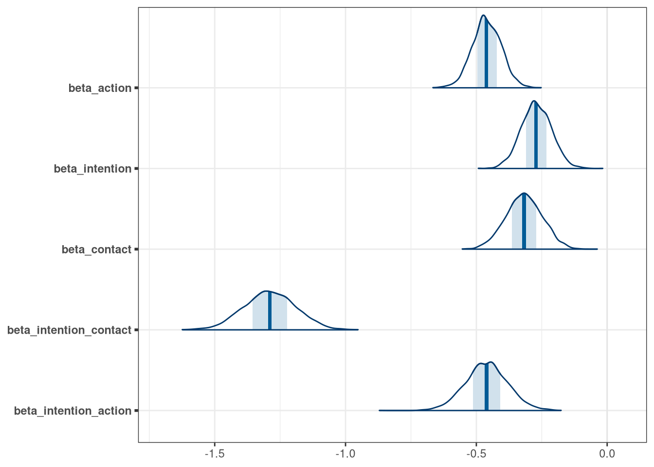
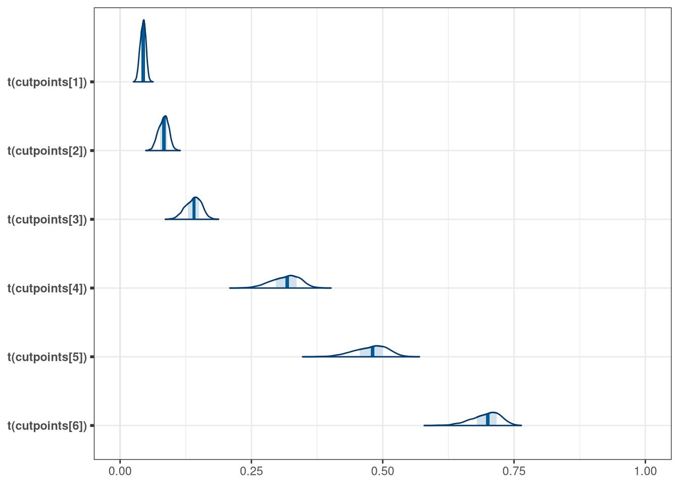
mcmc_areas(model1_interactions_draws, regex_pars = 'cut', transformations = inv.logit) + xlim(0, 1)## Scale for 'x' is already present. Adding another scale for 'x', which will
## replace the existing scale.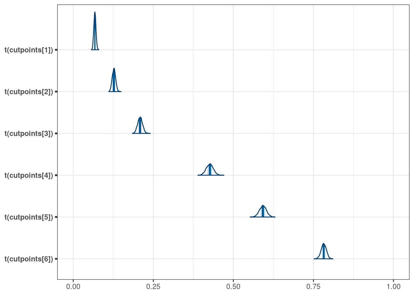
7.0.3 Model: ordered categorical predictors
Probability of data: \(R_{i} \sim \text{Ordered-logit}(\phi_{i}, K)\)
Linear model: \(\phi_{i} = \beta_{E} \sum_{j=0}^{E_{i}-1}\delta_{j} + \beta{A_{i}}A_{i} + \beta{I_{i}}I_{i} + \beta{C_{i}}C_{i}\)
Prior for each intercept: \(K_{k} \sim \text{Normal}(0, 1.5)\) Prior for each \(\beta\): \(\beta_{A}, \beta_{I}, \beta_{C}, \beta_{E}K_{k} \sim \text{Normal}(0, 1)\) Prior for the \(\delta\) vector: \(\delta \sim \text{Dirichlet}(\alpha)\)
Dirichlet distribution = multivariate extension of the beta distribution. Probabilities between zero and one, that all sum to one. It is parameterized by pseudo-counts of observations.
The intercept takes the first category, so we add 0 to the sequence of
Make sure to reorder education levels
writeLines(readLines(tar_read(stan_c_file_w07_model2)))## data {
## int N;
## int K;
## int N_edu;
## int response[N];
## int action[N];
## int intention[N];
## int contact[N];
## int education[N];
## vector[N_edu - 1] alpha;
## }
## parameters {
## // Cut points are the positions of responses along cumulative odds
## ordered[K] cutpoints;
## real beta_action;
## real beta_intention;
## real beta_contact;
## real beta_education;
##
## // Vector N reals that sum to 1
## simplex[7] delta;
## }
## model {
## vector[N] phi;
## vector[N_edu] delta_j;
##
## delta ~ dirichlet(alpha);
## delta_j = append_row(0, delta);
##
## for (i in 1:N) {
## // add beta education * sum delta j, up to current i's education
## phi[i] = beta_education * sum(delta_j[1:education[i]]) +
## beta_action * action[i] +
## beta_contact * contact[i] +
## beta_intention * intention[i];
## response[i] ~ ordered_logistic(phi[i], cutpoints);
## }
##
## cutpoints ~ normal(0, 1.5);
## beta_action ~ normal(0, 1);
## beta_contact ~ normal(0, 1);
## beta_intention ~ normal(0, 1);
## beta_education ~ normal(0, 1);
## }
model2_draws <- tar_read(stan_c_mcmc_w07_model2)$draws()

mcmc_areas(model2_draws, regex_pars = 'beta')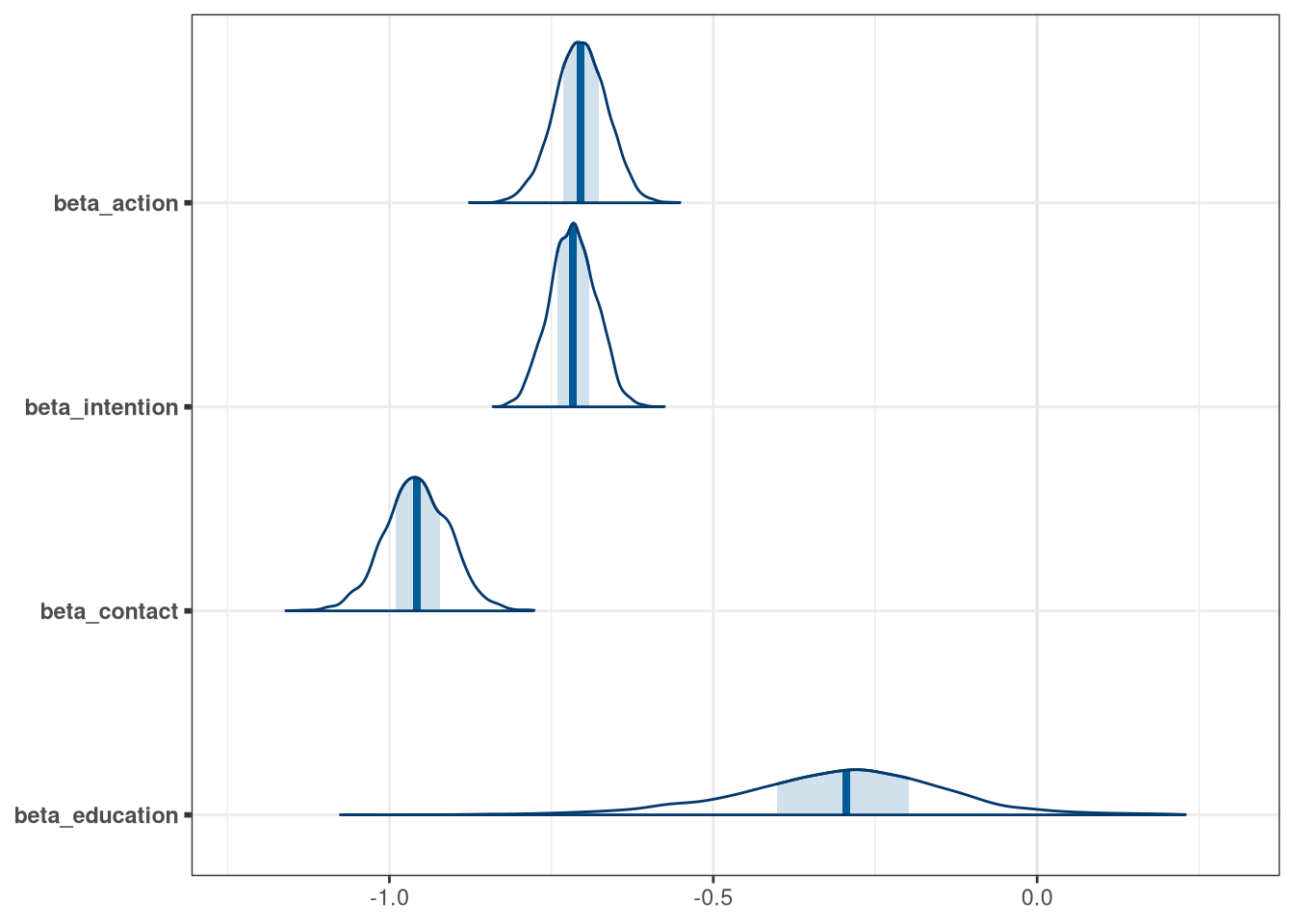
mcmc_areas(model2_draws, regex_pars = 'delta')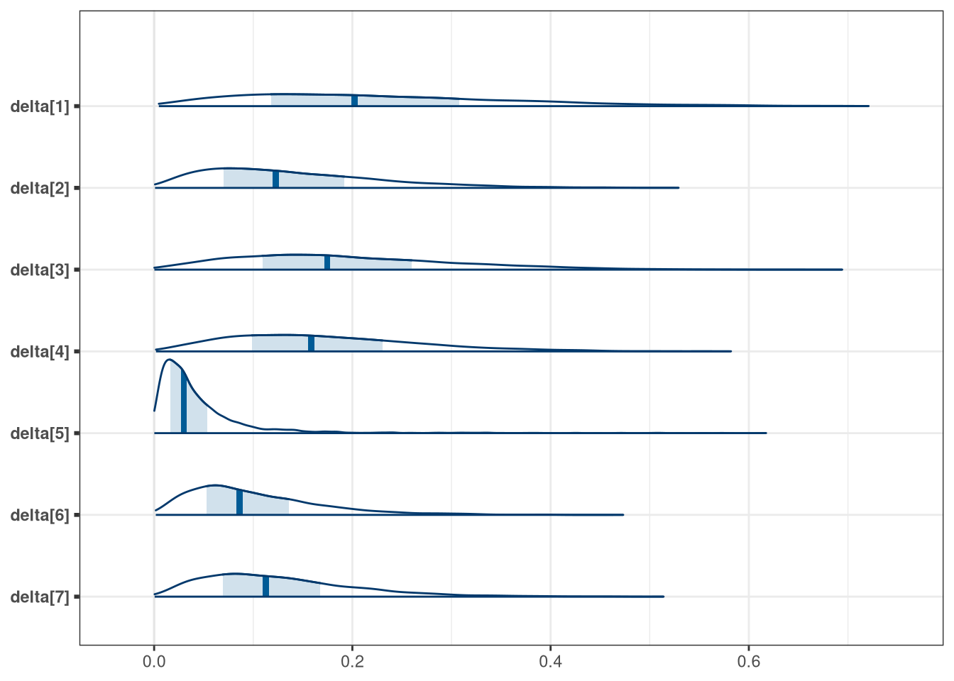
mcmc_areas(model2_draws, regex_pars = 'cut', transformations = inv.logit) + xlim(0, 1)## Scale for 'x' is already present. Adding another scale for 'x', which will
## replace the existing scale.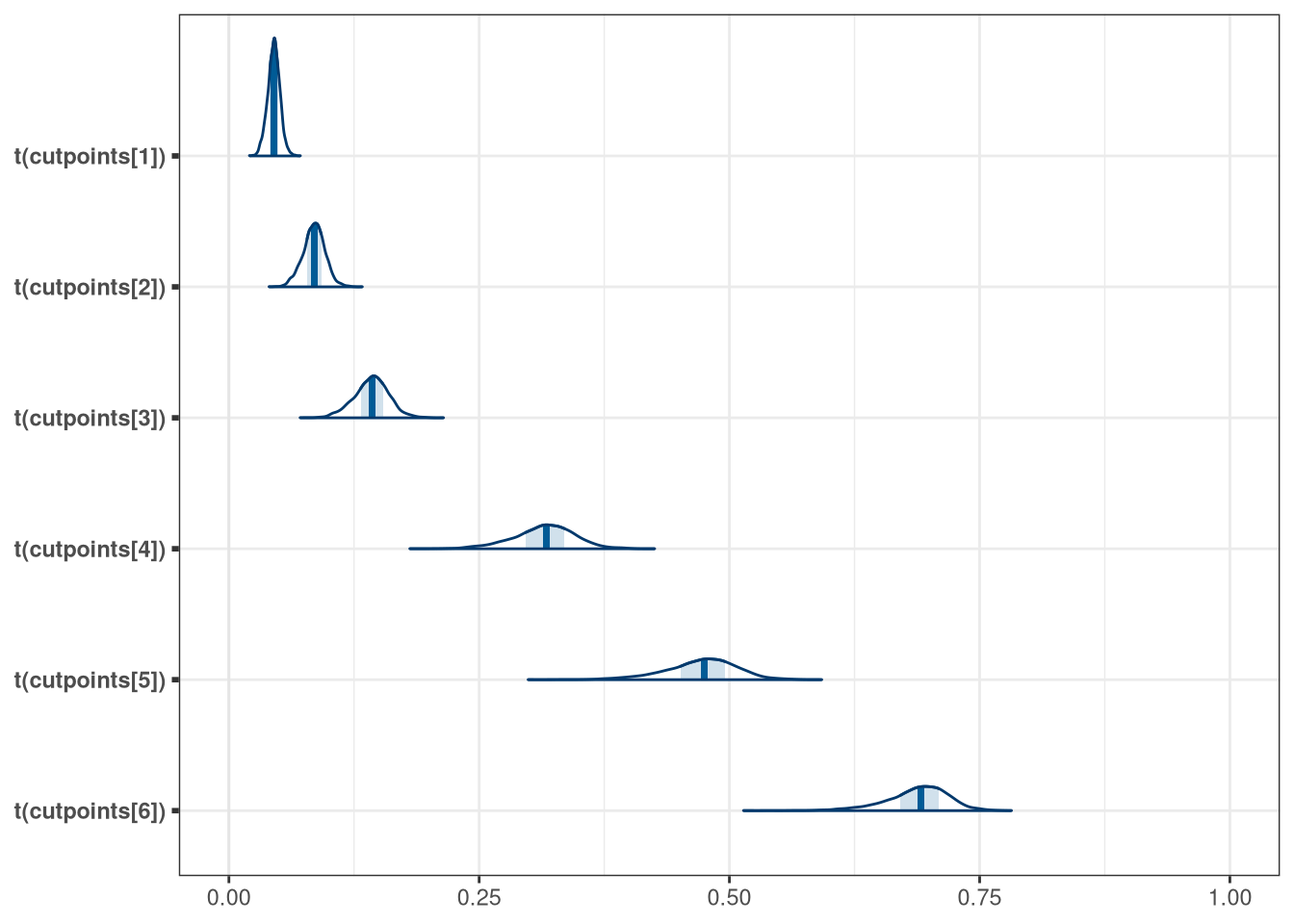
7.1 Question 1
In the Trolley data —
data(Trolley)— we saw how education level (modeled as an ordered category) is associated with responses. Is this association causal? One plausible confound is that education is also associated with age, through a causal process: People are older when they finish school than when they begin it. Reconsider the Trolley data in this light. Draw a DAG that represents hypothetical causal relationships among response, education, and age.
dag <- dagify(
  response ~ education + age + action + intention + contact,
  education ~ age,
  contact ~ action,
  exposure = 'education',
  outcome = 'response'
)

dag_plot(dag)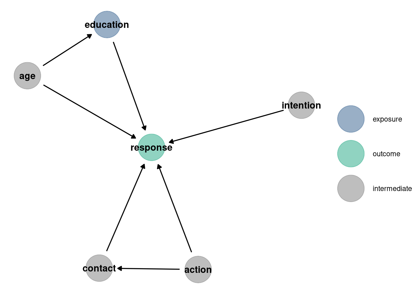
adjustmentSets(dag, exposure = 'education', outcome = 'response', effect = 'total' )## { age }Which statistical model or models do you need to evaluate the causal influence of education on responses? Fit these models to the trolley data. What do you conclude about the causal relationships among these three variables?
writeLines(readLines(tar_read(stan_c_file_w07_model2_age)))## data {
## int N;
## int K;
## int N_edu;
## int response[N];
## int action[N];
## int intention[N];
## int contact[N];
## int education[N];
## real age[N];
## vector[N_edu - 1] alpha;
## }
## parameters {
## // Cut points are the positions of responses along cumulative odds
## ordered[K] cutpoints;
## real beta_action;
## real beta_intention;
## real beta_contact;
## real beta_education;
## real beta_age;
##
## // Vector N reals that sum to 1
## simplex[7] delta;
## }
## model {
## vector[N] phi;
## vector[N_edu] delta_j;
##
## delta ~ dirichlet(alpha);
## delta_j = append_row(0, delta);
##
## for (i in 1:N) {
## // add beta education * sum delta j, up to current i's education
## phi[i] = beta_education * sum(delta_j[1:education[i]]) +
## beta_action * action[i] +
## beta_contact * contact[i] +
## beta_age * age[i] +
## beta_intention * intention[i];
## response[i] ~ ordered_logistic(phi[i], cutpoints);
## }
##
## cutpoints ~ normal(0, 1.5);
## beta_action ~ normal(0, 1);
## beta_contact ~ normal(0, 1);
## beta_intention ~ normal(0, 1);
## beta_education ~ normal(0, 1);
## beta_age ~ normal(0, 1);
## }
model2_age_draws <- tar_read(stan_c_mcmc_w07_model2_age)$draws()

mcmc_areas(model2_age_draws, regex_pars = 'beta')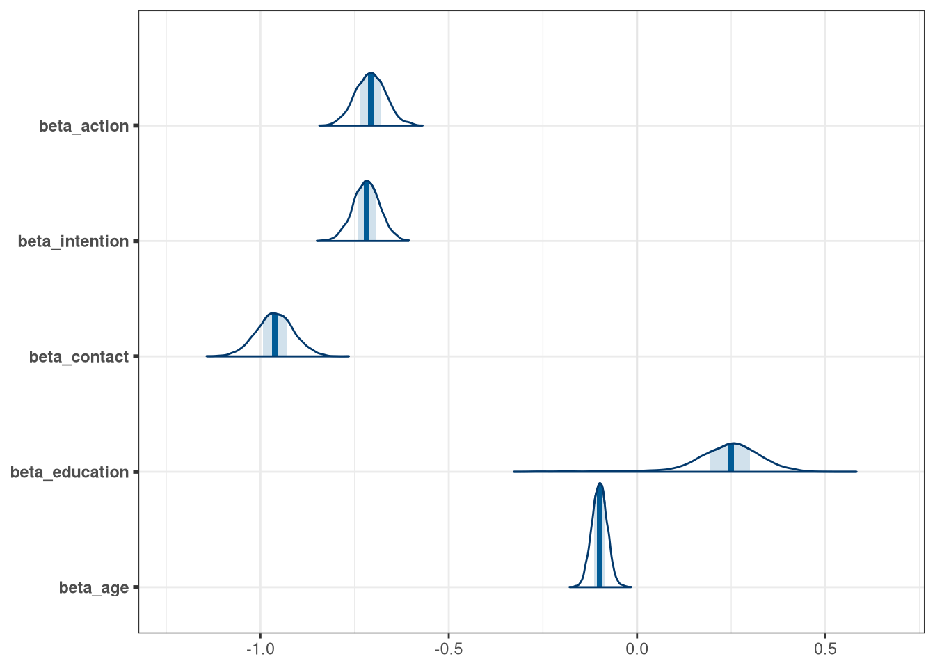
mcmc_areas(model2_age_draws, regex_pars = 'delta')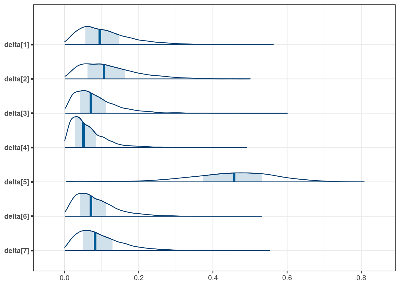
mcmc_areas(model2_age_draws, regex_pars = 'cut', transformations = inv.logit) + xlim(0, 1)## Scale for 'x' is already present. Adding another scale for 'x', which will
## replace the existing scale.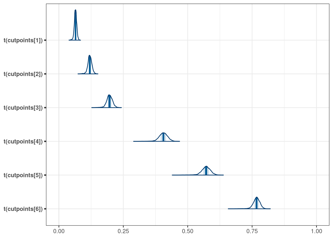
7.2 Question 2
Consider one more variable in the Trolley data: Gender. Suppose that gender might influence education as well as response directly. Draw the DAG now that includes response, education, age, and gender. Using only the DAG, is it possible that the inferences from Problem 1 are con founded by gender? If so, define any additional models you need to infer the causal influence of education on response. What do you conclude?
dag <- dagify(
  response ~ education + age + gender + action + intention + contact,
  education ~ age,
  education ~ gender,
  contact ~ action,
  exposure = 'education',
  outcome = 'response'
)

dag_plot(dag)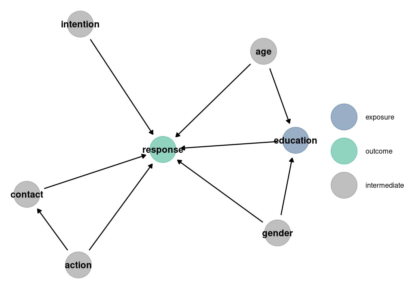
adjustmentSets(dag, exposure = 'education', outcome = 'response', effect = 'total' )## { age, gender }
writeLines(readLines(tar_read(stan_c_file_w07_model2_gender)))## data {
## int N;
## int K;
## int N_edu;
## int response[N];
## int action[N];
## int intention[N];
## int contact[N];
## int education[N];
## real age[N];
## int gender[N];
## vector[N_edu - 1] alpha;
## }
## parameters {
## // Cut points are the positions of responses along cumulative odds
## ordered[K] cutpoints;
## real beta_action;
## real beta_intention;
## real beta_contact;
## real beta_education;
## real beta_age;
## real beta_gender;
##
## // Vector N reals that sum to 1
## simplex[7] delta;
## }
## model {
## vector[N] phi;
## vector[N_edu] delta_j;
##
## delta ~ dirichlet(alpha);
## delta_j = append_row(0, delta);
##
## for (i in 1:N) {
## // add beta education * sum delta j, up to current i's education
## phi[i] = beta_education * sum(delta_j[1:education[i]]) +
## beta_action * action[i] +
## beta_contact * contact[i] +
## beta_age * age[i] +
## beta_gender * gender[i] +
## beta_intention * intention[i];
## response[i] ~ ordered_logistic(phi[i], cutpoints);
## }
##
## cutpoints ~ normal(0, 1.5);
## beta_action ~ normal(0, 1);
## beta_contact ~ normal(0, 1);
## beta_intention ~ normal(0, 1);
## beta_education ~ normal(0, 1);
## beta_age ~ normal(0, 1);
## beta_gender ~ normal(0, 1);
## }
model2_gender_draws <- tar_read(stan_c_mcmc_w07_model2_gender)$draws()

mcmc_areas(model2_gender_draws, regex_pars = 'beta')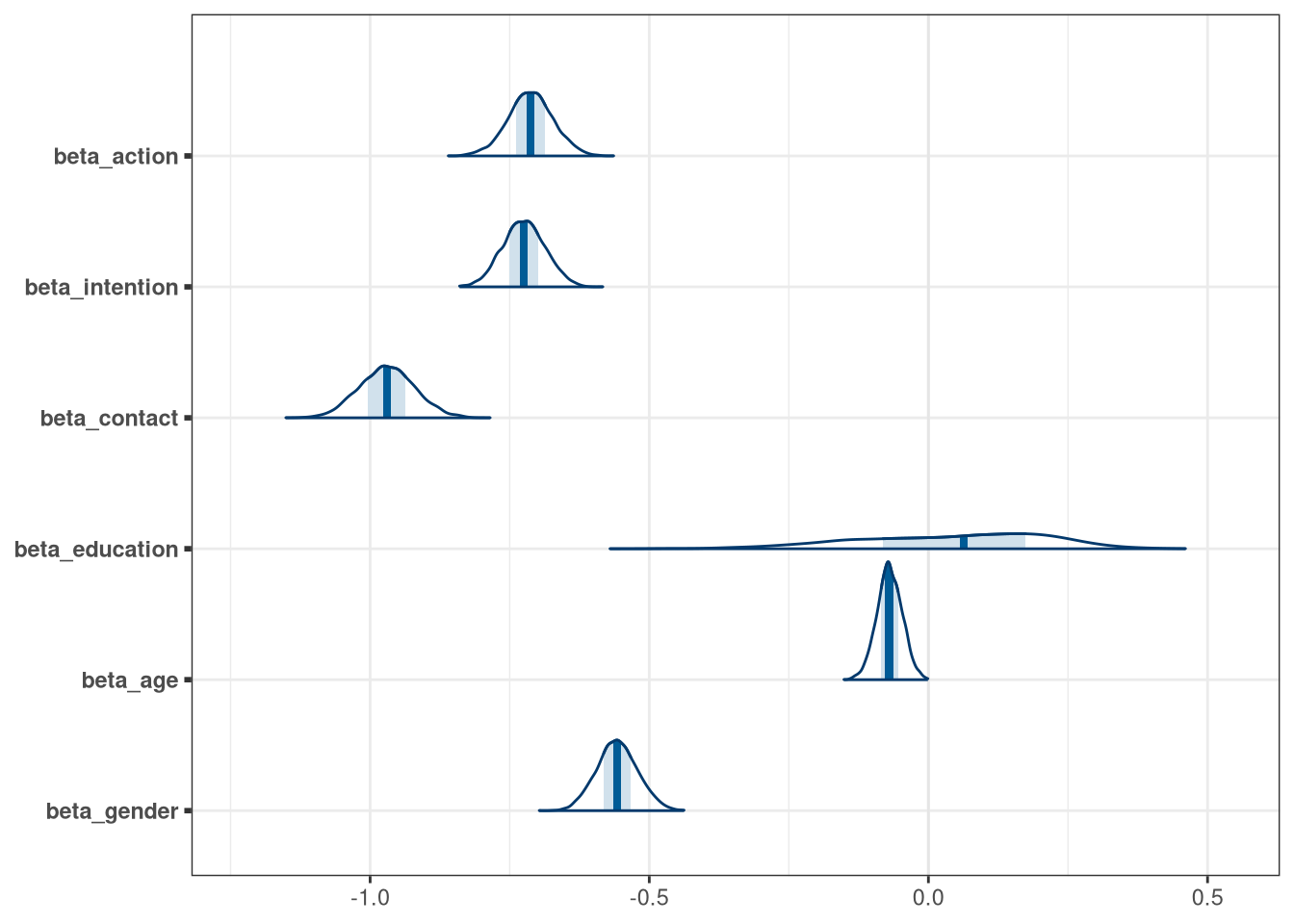
mcmc_areas(model2_gender_draws, regex_pars = 'delta')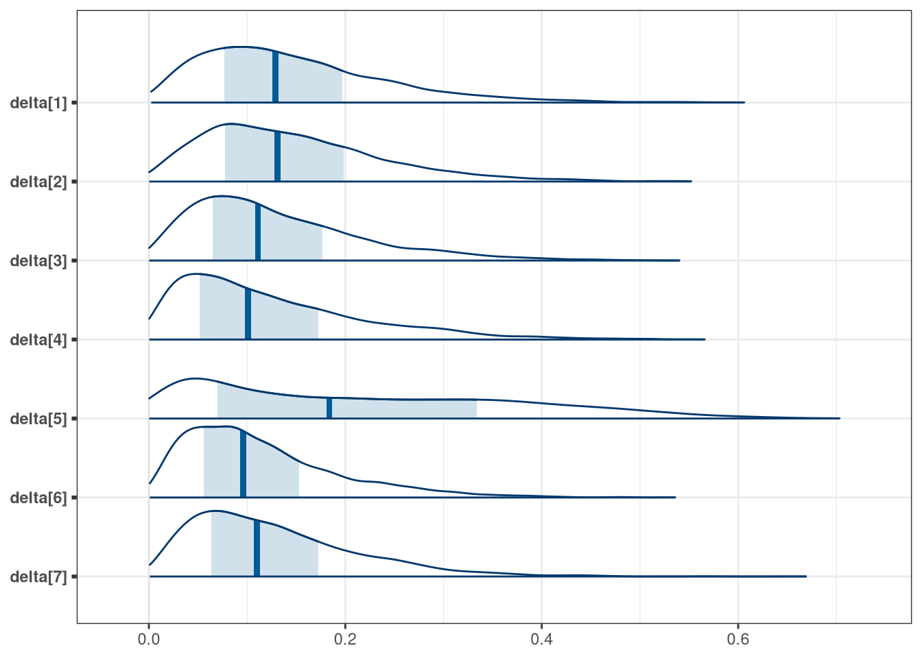
mcmc_areas(model2_gender_draws, regex_pars = 'cut', transformations = inv.logit) + xlim(0, 1)## Scale for 'x' is already present. Adding another scale for 'x', which will
## replace the existing scale.